8 Low-Rank method

Low-Rank Methods for Parallelizing Dynamic Programming Algorithms

PDF

SAEED MALEKI, University of Illinois at Urbana-Champaign
MADANLAL MUSUVATHI and TODD MYTKOWICZ, Microsoft Research

This article proposes efficient parallel methods for an important class of dynamic programming problems that includes Viterbi, Needleman-Wunsch, Smith-Waterman, and Longest Common Subsequence. In dynamic programming, the subproblems that do not depend on each other, and thus can be computed in parallel, form stages or wavefronts. The methods presented in this article provide additional parallelism allowing multiple stages to be computed in parallel despite dependencies among them. The correctness and the performance of the algorithm relies on rank convergence properties of matrix multiplication in the tropical semiring, formed with plus as the multiplicative operation and max as the additive operation.

This article demonstrates the efficiency of the parallel algorithm by showing significant speedups on a variety of important dynamic programming problems. In particular, the parallel Viterbi decoder is up to $24\times$ faster (with 64 processors) than a highly optimized commercial baseline.

CCS Concepts: $\bullet$ Theory of computation $\rightarrow$ Parallel algorithms; $\bullet$ Computing methodologies $\rightarrow$ Concurrent algorithms;

Additional Key Words and Phrases: Parallelism, dynamic programming, tropical semiring, longest common subsequence, Needleman-Wunsch

Saeed Maleki, Madanlal Musuvathi, and Todd Mytkowicz. 2016. Low-rank methods for parallelizing dynamic programming algorithms. ACM Trans. Parallel Comput. 2, 4, Article 26 (February 2016), 32 pages. DOI: http://dx.doi.org/10.1145/2884065

1. INTRODUCTION

Dynamic programming [Bellman 1957] is an approach to solve a variety of important optimization problems in computer science, economics, genomics, and finance. Figure 1 describes two such examples: Viterbi, which finds the most likely path through a hidden Markov model for a sequence of observations, and Longest Common Subsequence (LCS), which finds the longest common subsequence between two input strings. Dynamic programming algorithms proceed by recursively solving a series of subproblems, usually represented as cells in a table, as shown in the figure. The solution to a subproblem is constructed from solutions to an appropriate set of subproblems, as shown by the respective recurrence relation in the figure.

These data dependencies naturally group subproblems into stages whose solutions do not depend on each other. For example, all subproblems in a column form a stage in Viterbi, and all subproblems in an antidiagonal form a stage in LCS. A predominant method for parallelizing dynamic programming is wavefront parallelization [Muraoka 1971], which computes all subproblems within a stage in parallel¹.

¹The definition of wavefront parallelism used here is more general and includes the common usage where a wavefront performs computations across logical iterations as in the LCS example in Figure 1(a).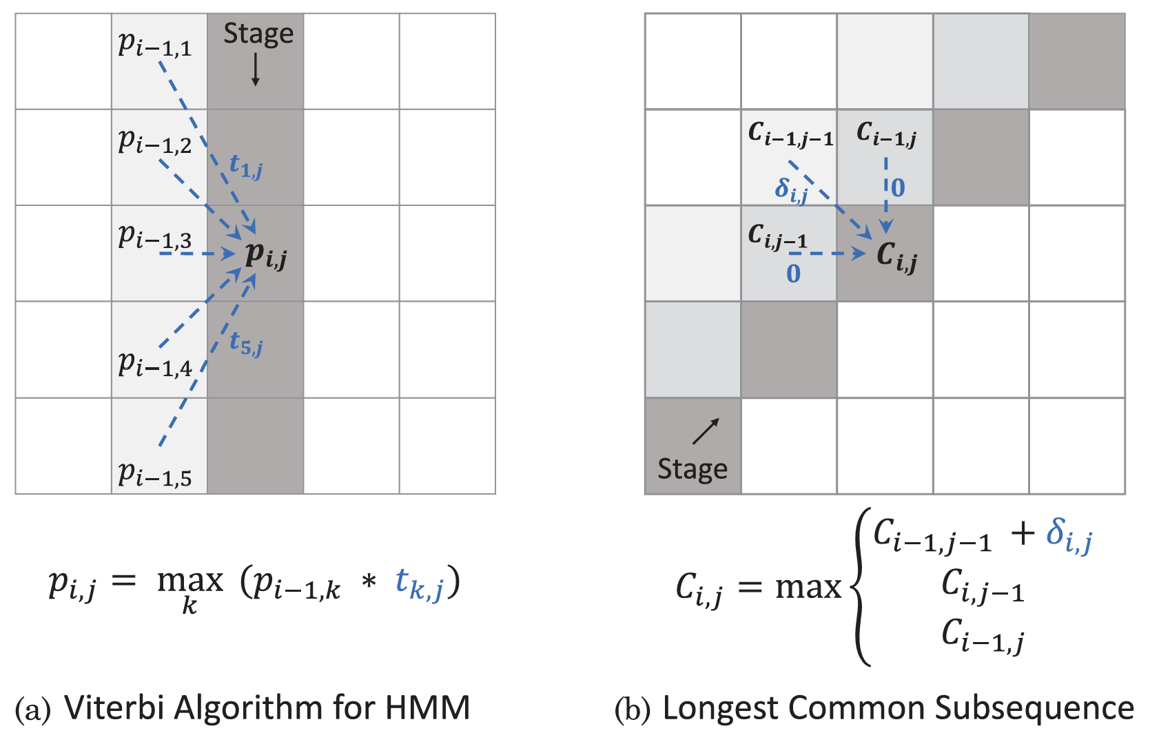

Fig. 1. Dynamic programming examples with dependencies between stages. (a) The Viterbi algorithm for finding the most likely path in a hidden Markov model (HMM). (b) The Longest Common Subsequence (LCS) algorithm, which searches for the best subsequence shared between two strings.

In contrast, this article breaks data dependencies across stages and fixes up incorrect values later in the algorithm. Therefore, this approach exposes parallelism for a class of dynamic programming algorithms we call linear-tropical dynamic programming (LTDP). An LTDP computation can be viewed as performing a sequence of matrix multiplications in the tropical semiring where the semiring is formed with $+$ as the multiplicative operator and max as the additive operator. This article demonstrates that several important optimization problems such as Viterbi, LCS, Smith-Waterman, and Needleman-Wunsch (the latter two are used in bioinformatics for sequence alignment) belong to LTDP. To efficiently break data dependencies across stages, the algorithm uses rank convergence, a property by which the rank of a sequence of matrix products in the tropical semiring is likely to converge to a low rank (or rank 1 in many cases).

A key advantage of our parallel methods is the ability to simultaneously use both the coarse-grained parallelism across stages and the fine-grained wavefront parallelism within a stage. Moreover, the algorithm can reuse existing highly optimized implementations that exploit wavefront parallelism with little modification. As a consequence, our implementation achieves multiplicative speedups over existing implementations. For instance, the parallel Viterbi decoder is up to $24\times$ faster with 64 cores than a state-of-the-art commercial baseline [Puschel et al. 2005]. This article demonstrates similar speedups for other LTDP instances studied in this article.

2. BACKGROUND

In linear algebra, a matrix-vector multiplication maps a vector from an input space to an output space. If the matrix is of low rank, the matrix maps the vector to a subspace of the output space. In particular, if the matrix has rank 1, then it maps all input vectors to a line in the output space. These geometric intuitions hold even when one changes the meaning of the sum and multiplication operators (say, to max and $+$ , respectively), as long as the new meaning satisfies the following rules.

Semirings. A semiring is a five-tuple $(D,\oplus ,\otimes , 𝟘, 𝟙)$ , where $D$ is the domain of the semiring that is closed under the additive operation $\oplus$ and the multiplicative operation $\otimes$ . The two operations satisfy the following properties:

• $(D,\oplus ,𝟘)$ forms a commutative monoid with $𝟘$ as the identity
  • associativity: $\forall x,y,z\in D:(x\oplus y)\oplus z = x\oplus (y\oplus z)$
  • identity: $\forall x\in D:x\oplus 𝟘 = x$
  • commutativity: $\forall x,y\in D:x\oplus y = y\oplus x$
• $(D,\otimes ,𝟙)$ forms a monoid with $𝟙$ as the identity
  • associativity: $\forall x,y,z\in D:(x\otimes y)\otimes z = x\otimes (y\otimes z)$
  • identity: $\forall x\in D:x\otimes 𝟙 = 𝟙\otimes x = x$
• $\otimes$ left- and right-distributes over $\oplus$
  • $\forall x,y,z\in D:x\otimes (y\oplus z) = (x\otimes y)\oplus (x\otimes z)$
  • $\forall x,y,z\in D:(y\oplus z)\otimes x = (y\otimes x)\oplus (z\otimes x)$
• $𝟘$ is an annihilator for $\otimes$
  • $\forall x\in D:x\otimes 𝟘 = 𝟘 \otimes x = 𝟘$

Tropical Semiring. The semiring $(\mathbb{R}\cup \{-\infty \} ,\max , + , - \infty ,0)$ with the real numbers extended with $-\infty$ as the domain, max as the additive operation $\oplus$, and $+$ as the multiplicative operation $\otimes$ is called the tropical semiring. All properties of a semiring hold with $-\infty$ as the additive identity $𝟘$ and $0$ as the multiplicative identity $𝟙$ . Alternately, one can reverse the sign of every element in the domain and change the additive operation to min.

Matrix Multiplication. Let $A_{n\times m}$ denote a matrix with $n$ rows and $m$ columns with elements from the domain of the tropical semiring. Let $A[i,j]$ denote the element of $A$ at the $i$th row and $j$th column. The matrix product of $A_{l\times m}$ and $B_{m\times n}$ is $A\odot B$ , a $l\times n$ matrix defined such that

$$(A\odot B)[i,j] = \bigoplus_{1\leq k\leq m}(A[i,k]\otimes B[k,j])$$ $$= \max_{1\leq k\leq m}(A[i,k] + B[k,j]).$$

Note, this is the standard matrix product with multiplication replaced by $+$ and addition replaced by max.

The transpose of $A_{n\times m}$ is the matrix $A_{m\times n}^{\mathrm{T}}$ such that $\forall i,j:A^{\mathrm{T}}[i,j] = A[j,i]$ . Using standard terminology, we will denote a $v_{n\times 1}$ matrix as the column vector $\vec{v}$ , a $v_{1\times n}$ matrix as the row vector $\vec{v}^{\mathrm{T}}$ , and a $x_{1\times 1}$ matrix simply as the scalar $x$ . This terminology allows us to extend the definition of matrix-matrix multiplication above to matrix-vector, scalar-matrix, and scalar-vector multiplication appropriately. Also, $\vec{v} [i]$ is the $i$th element of a vector $\vec{v}$ . The following lemma follows from the associativity, distributivity, and commutativity properties of $\otimes$ and $\oplus$ in a semiring.

LEMMA 2.1. Matrix multiplication is associative in semirings

$$(A\odot B)\odot C = A\odot (B\odot C).$$

Parallel Vectors. Two vectors $\vec{u}$ and $\vec{v}$ are parallel in the tropical semiring, denoted as $\vec{u}\parallel \vec{v}$ , if there exist scalars $x$ and $y$ such that $\vec{u}\odot x = \vec{v}\odot y$ . Intuitively, parallel vectors in tropical semiring $\vec{u}$ and $\vec{v}$ differ by a constant offset. For instance, $[1, 0, 2]^{\mathrm{T}}$ and $[3, 2, 4]^{\mathrm{T}}$ are parallel vectors differing by an offset 2. Note that the previous definition requires the two scalars not to be $-\infty$ as $-\infty$ does not have a multiplicative inverse in the tropical semiring.

Matrix Rank. The rank of a matrix $M_{m\times n}$ , denoted by $\operatorname{rank}(M)$ , is the smallest number $r$ such that there exist matrices $C_{m\times r}$ and $R_{r\times n}$ whose product is $M$ . In particular, a rank-1 matrix is a product of a column vector and a row vector. There are alternate ways to define the rank of a matrix in semirings, such as the number of linearly independent rows or columns in a matrix. While such definitions coincide in fields (which have inverses for $\oplus$ and $\otimes$ ), they are not equivalent in semirings [Develin et al. 2005].

LEMMA 2.2. For any vectors $\vec{u}$ and $\vec{v}$ and a matrix $A$ of rank 1, $A\odot \vec{u}\parallel A\odot \vec{v}$

Intuitively, this lemma states that a rank-1 matrix maps all vectors to a line. If $\operatorname{rank}(A) = 1$ , then it is a product of some column vector $\vec{c}$ and a row vector $\vec{r}^{\intercal}$ . For any vectors $\vec{u}$ and $\vec{v}$ ..

$$A\odot \vec{u} = (\vec{c}\odot \vec{r}^{\intercal})\odot \vec{u} = \vec{c}\odot (\vec{r}^{\intercal}\odot \vec{u}) = \vec{c}\odot x_{u}$$ $$A\odot \vec{v} = (\vec{c}\odot \vec{r}^{\intercal})\odot \vec{v} = \vec{c}\odot (\vec{r}^{\intercal}\odot \vec{v}) = \vec{c}\odot x_{v}$$

for appropriate scalars $x_{u}$ and $x_{v}$ . As an example, consider

$$A = \begin{bmatrix} 1 & 2 & 3 \\ 2 & 3 & 4 \\ 3 & 4 & 5 \end{bmatrix} \qquad \vec{u} = \begin{bmatrix} 1 \\ -\infty \\ 3 \end{bmatrix} \qquad \vec{v} = \begin{bmatrix} -\infty \\ 2 \\ 0 \end{bmatrix}.$$

$A = [1, 2, 3]^\top \odot [0, 1, 2]$ is rank-1. $A\odot \vec{u} = [6, 7, 8]^{\intercal}$ and $A\odot \vec{v} = [4, 5, 6]^{\intercal}$ , which are parallel with a constant offset 2. Also note that all rows in a rank-1 matrix are parallel to each other.

---

Max-Plus: A

$$A = \begin{bmatrix} 1 \\ 2 \\ 3 \end{bmatrix} \otimes \begin{bmatrix} 0 & 1 & 2 \end{bmatrix} = \begin{bmatrix} 1+0 & 1+1 & 1+2 \\ 2+0 & 2+1 & 2+2 \\ 3+0 & 3+1 & 3+2 \end{bmatrix} = \begin{bmatrix} 1 & 2 & 3 \\ 2 & 3 & 4 \\ 3 & 4 & 5 \end{bmatrix}$$

Max-Plus: $A\odot \vec{u}$

$$A\odot \vec{u} = \begin{bmatrix} 1 \\ 2 \\ 3 \end{bmatrix} \otimes \begin{bmatrix} 0 & 1 & 2 \end{bmatrix} \otimes \begin{bmatrix} 6 \\ 7 \\ 8 \end{bmatrix} = \begin{bmatrix} 6 \\ 7 \\ 8 \end{bmatrix}$$

$inner\ product: [0, 1, 2] \otimes \begin{bmatrix} 1 \\ -\infty \\ 3 \end{bmatrix} = \max(0+1,\ 1+(-\infty),\ 2+3) = \max(1,\ -\infty,\ 5) = 5$

$scalar\ product: \begin{bmatrix} 1 \\ 2 \\ 3 \end{bmatrix} \otimes 5 = \begin{bmatrix} 1+5 \\ 2+5 \\ 3+5 \end{bmatrix} = \begin{bmatrix} 6 \\ 7 \\ 8 \end{bmatrix}$

Max-Plus: $A\odot \vec{v}$

$$A\odot \vec{v} = \begin{bmatrix} 1 \\ 2 \\ 3 \end{bmatrix} \otimes [0, 1, 2] \otimes \begin{bmatrix} -\infty \\ 2 \\ 0 \end{bmatrix} = \begin{bmatrix} 4 \\ 5 \\ 6 \end{bmatrix}$$

$inner\ product: [0, 1, 2] \otimes \begin{bmatrix} -\infty \\ 2 \\ 0 \end{bmatrix} = \max(0+(-\infty),\ 1+2,\ 2+0) = \max(-\infty,\ 3,\ 2) = 3$

$scalar\ product: \begin{bmatrix} 1 \\ 2 \\ 3 \end{bmatrix} \otimes 3 = \begin{bmatrix} 1+3 \\ 2+3 \\ 3+3 \end{bmatrix} = \begin{bmatrix} 4 \\ 5 \\ 6 \end{bmatrix}$

linear algebra：

$$\begin{bmatrix} 1 \\ 2 \\ 3 \end{bmatrix} \begin{bmatrix} 0 & 1 & 2 \end{bmatrix} = \begin{bmatrix} 1\times0 & 1\times1 & 1\times2 \\ 2\times0 & 2\times1 & 2\times2 \\ 3\times0 & 3\times1 & 3\times2 \end{bmatrix} = \begin{bmatrix} 0 & 1 & 2 \\ 0 & 2 & 4 \\ 0 & 3 & 6 \end{bmatrix}$$$$\begin{bmatrix} 1 \\ 2 \\ 3 \end{bmatrix} \begin{bmatrix} 0 & 1 & 2 \end{bmatrix} \begin{bmatrix} 1 \\ -\infty \\ 3 \end{bmatrix} = (0 - \infty + 6) \begin{bmatrix} 1 \\ 2 \\ 3 \end{bmatrix} = \begin{bmatrix} -\infty \\ -\infty \\ -\infty \end{bmatrix}$$$$\begin{bmatrix} 1 \\ 2 \\ 3 \end{bmatrix} \begin{bmatrix} 0 & 1 & 2 \end{bmatrix} \begin{bmatrix} -\infty \\ 2 \\ 0 \end{bmatrix} = (0 + 2 + 0) \begin{bmatrix} 1 \\ 2 \\ 3 \end{bmatrix} = \begin{bmatrix} 2 \\ 4 \\ 6 \end{bmatrix}$$

3. LINEAR-TROPICAL DYNAMIC PROGRAMMING

Dynamic programming is an approach for solving problems that have optimal substructure - the solution to a problem can be obtained from the solutions to a set of its overlapping subproblems. This dependence between subproblems is captured by a recurrence equation. Classic dynamic programming implementations solve the subproblems iteratively, applying the recurrence equation in an order that respects the dependence between subproblems.

LTDP Definition. A dynamic programming problem is LTDP, if (1) the subproblems can be grouped into a sequence of stages such that the solution to a subproblem in a stage only depends on the solutions in the previous stage, and (2) this dependence is linear in the tropical semiring. In other words, $s_i[j]$ , the solution to subproblem $j$ in stage $i$ of LTDP, is given by the recurrence equation

$$s_i[j] = \max_{k}(s_{i - 1}[k] + A_i[j,k]) \quad (1)$$

for appropriate constants $A_i[j,k]$ . This linear dependence allows us to view LTDP as computing a sequence of vectors $\vec{s}_1, \vec{s}_2, \ldots , \vec{s}_n$ , where

$$\vec{s}_i = A_i\odot \vec{s}_{i - 1} \quad (2)$$

for an appropriate matrix of constants $A_i$ derived from the recurrence equation. In this equation, we will call $\vec{s}_i$ the solution vector at stage $i$ and call $A_i$ the transformation matrix at stage $i$ . Also, $\vec{s}_0$ is the initial solution vector obtained from the base case of the recurrence equation.

Predecessor Product. Once all of the subproblems are solved, finding the solution to the underlying optimization problem of LTDP usually involves tracing the predecessors of subproblems. A predecessor of a subproblem is the subproblem for which the maximum in Equation (1) is reached. For ease of exposition, we define the predecessor product of a matrix $A$ and a vector $\vec{s}$ as the vector $A\star \vec{s}$ such that

$$(A\star \vec{s})[j] = \arg \max_{k}(\vec{s}[k] + A[j,k]).$$

Note the similarity between this definition and Equation (1). We assume that ties in arg max are broken deterministically. The following lemma shows that predecessor products do not distinguish between parallel vectors, a property that will be useful later.

LEMMA 3.1. $\vec{u}\parallel \vec{v} ⇒ \forall A:A\star \vec{u} = A\star \vec{v}.$

This follows from the fact that parallel vectors in the tropical semiring differ by a constant and that arg max is invariant when a constant is added to all its arguments.

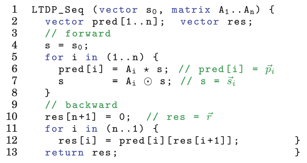
Fig. 2. LTDP implementation that computes the stages sequentially. An implementation can possibly employ wavefront parallelization within a stage.

Sequential LTDP. Figure 2 shows the sequential algorithm for LTDP phrased in terms of matrix multiplications and predecessor products. This algorithm is deemed sequential because it computes the stages one after the other based on the data dependence in Equation (1). However, the algorithm can utilize wavefront parallelism to compute the solutions within a stage in parallel.

The inputs to the sequential algorithm are the initial solution vector $\vec{s}_0$ and transformation matrices $A_1, \ldots , A_n$ , which respectively capture the base and inductive case of the LTDP recurrence equation. The algorithm consists of a forward phase and a backward phase. The forward phase computes the solutions in each stage $\vec{s}_i$ iteratively. In addition, it computes the predecessor product $\vec{p}_i$ that determines the predecessor for each solution in a stage. The backward phase iteratively follows the predecessors computed in the forward phase. The algorithm assumes that the first subproblem in the last stage, $\vec{v}_n[0]$ , contains the desired solution to the underlying optimization problem. Accordingly, the backward phase starts with 0 in Line 10. The resulting vector res is the solution to the optimization problem at hand (e.g., the longest common subsequence of the two input strings).

The previous exposition consciously hides a lot of details in the $\odot$ and $\star$ operators. An implementation does not need to represent the solutions in a stage as a vector and perform matrix-vector operations. It might statically know that the current solution depends on some of the subproblems in the previous stage (a sparse matrix) and only access those. Finally, as mentioned earlier, an implementation might use wavefront parallelism to compute the solutions in a stage in parallel. All these implementation details are orthogonal to how the parallel algorithm described in this article parallelizes across stages.

4. THE PARALLEL RANK-1 METHOD

This section describes the Rank-1 method for parallelizing the sequential algorithm in Figure 2 across stages.

4.1. Breaking Data Dependencies Across Stages

Viewing LTDP computation as matrix multiplication in the tropical semiring provides a way to break data dependencies among stages. Consider the solution vector at the last stage $\bar{s}_n$ . From Equation (2), we have

$\bar{s}_n = A_n\odot A_{n - 1}\ldots A_2\odot A_1\odot \bar{s}_0.$

Standard techniques [Ladner and Fischer 1980; Hillis and Steele 1986] can parallelize this computation using the associativity of matrix multiplication. For instance, two processors can compute the partial products $A_n\odot \ldots \odot A_{n / 2 + 1}$ and $A_{n / 2}\odot \ldots \odot A_{1}$ in parallel and multiply their results with $\bar{s}_0$ to obtain $\bar{s}_n$ .

However, doing so converts a sequential computation that performs matrix-vector multiplications to a parallel computation that performs matrix-matrix multiplications. This results in a parallelization overhead linear in the size of the stages and thus requires a linear number of processors to observe constant speedups. In practice, the size of stages can easily be hundreds or larger and thus this is not practical on real problems and hardware.

The key contributions of this article are parallel methods that avoid the overhead of matrix-matrix multiplications. This section introduces the Rank-1 method that relies on the convergence of matrix rank to 1 in the tropical semiring as discussed later. Its exposition requires the following definition.

Partial Product. For a given LTDP instance, the partial product $M_{i \to j}$ , defined for stages $j \geq i$ , is given by

$M_{i\to j} = A_{j}\odot \ldots A_{i + 1}\odot A_{i}.$

Partial product determines how a later stage $j$ depends on stage $i$ as $\bar{s}_j = M_{i \to j} \odot \bar{s}_i$ .

4.2. Rank Convergence

Rank of the product of two matrices is not greater than the rank of the individual matrices:

$$\mathrm{rank}(A\odot B)\leq \min (\mathrm{rank}(A),\mathrm{rank}(B)). \quad (3)$$

This is because, if $\mathrm{rank}(A) = r$ , then $A = C \odot R$ for some matrix $C$ with $r$ columns. Thus, $A \odot B = (C \odot R) \odot B = C \odot (R \odot B)$ , implying that $\mathrm{rank}(A \odot B) \leq \mathrm{rank}(A)$ . Similar argument shows that $\mathrm{rank}(A \odot B) \leq \mathrm{rank}(B)$ .

Equation (3) implies that for stages $k \geq j \geq i$ ,

$$\mathrm{rank}(M_{i \to k}) \leq \mathrm{rank}(M_{i \to j}) \leq \mathrm{rank}(A_i).$$

In effect, as the LTDP computation proceeds, the rank of the partial products will never increase. Theoretically, there is a possibility that the ranks do not decrease. However, we have only observed this for carefully crafted problem instances that are unlikely to occur in practice. On the contrary, the rank of these partial products is likely to converge to 1, as will be demonstrated in Section 7.1.

Consider a partial product $M_{i \to j}$ whose rank is 1. Intuitively, this implies a weak dependence between stages $i$ and $j$ . Instead of the actual solution vector, $\bar{s}_i$ , say the LTDP computation starts with a different vector $\bar{t}_i$ at stage $i$ . From Lemma 2.2, the new solution vector at stage $j$ , $\bar{t}_j = M_{i \to j} \odot \bar{t}_i$ , is parallel to the actual solution vector $\bar{s}_j = M_{i \to j} \odot \bar{s}_i$ . Essentially, the direction of the solution vector at stage $j$ is independent of stage $i$ . The latter stage only determines its magnitude. In the tropical semiring, where the multiplicative operator is $+$ , this means that the solution vector at stage $j$ will be off by a constant if one starts stage $i$ with an arbitrary vector.

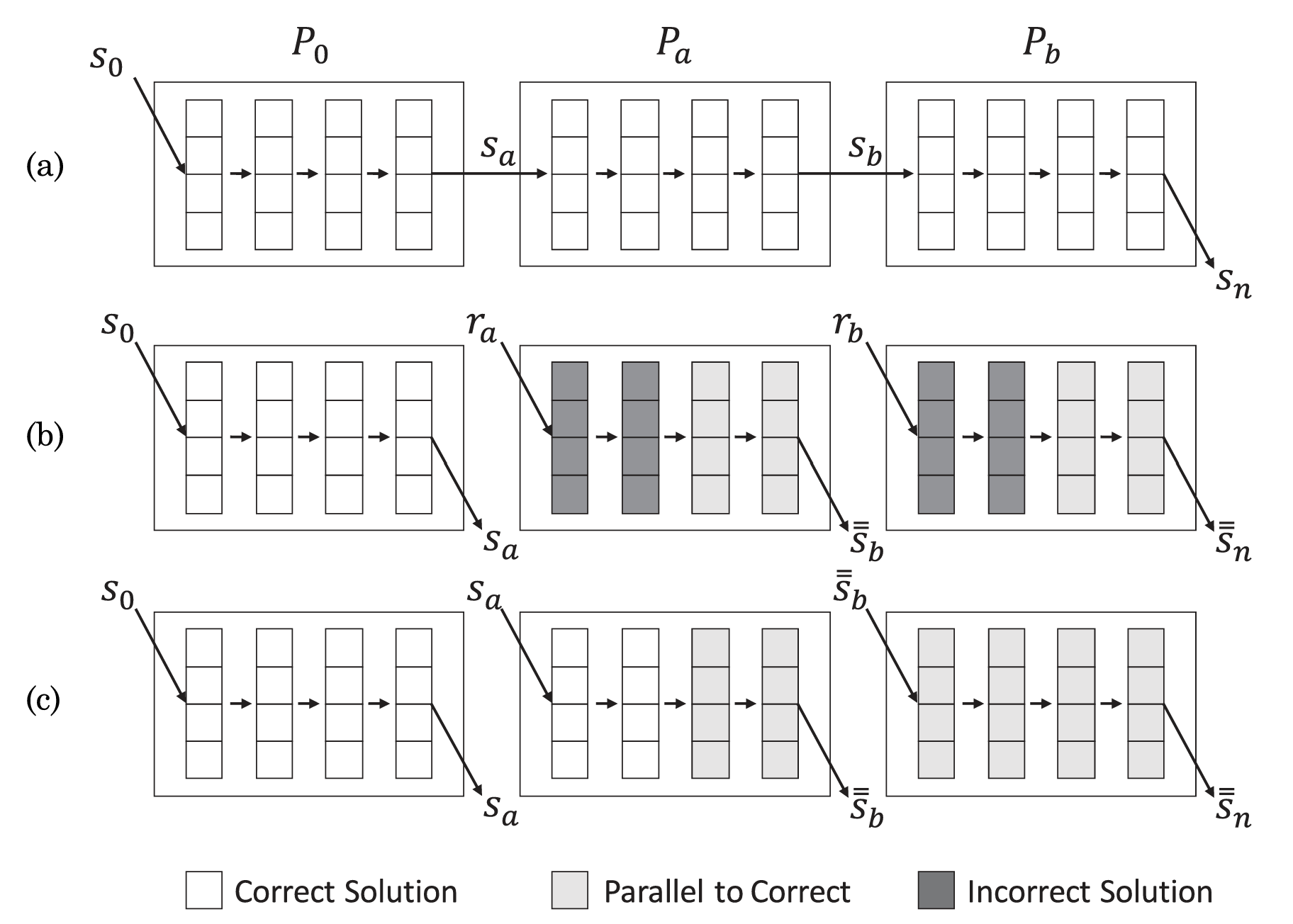
Fig. 3. Parallel algorithm for the forward phase of the sequential algorithm in Figure 2 using rank convergence. (a) The sequential algorithm. (b) The first phase of the parallel algorithm using arbitrary solutions. (c) The fix-up phase of the parallel algorithm.

4.3. The Rank-1 Method Overview

The Rank-1 method uses this insight to break dependencies between stages as shown pictorially in Figure 3. The figure uses three processors as an example. Figure 3(a) represents the forward phase of the sequential algorithm described in Figure 2. Each stage is represented as a vertical column of cells, and an arrow between stages represents a multiplication with an appropriate transformation matrix. Processor $P_0$ starts from the initial solution vector $s_0$ and computes all its stages. Processor $P_a$ waits for $s_a$ the solution vector in the final stage of $P_0$ , in order to start its computation. Similarly, processor $P_b$ waits for $s_b$ , the solution vector, at the final stage of $P_a$ .

In the parallel algorithm shown in Figure 3(b), processors $P_a$ and $P_b$ start from arbitrary solutions $r_a$ and $r_b$ , respectively, in parallel with $P_0$ . Of course, the solutions for the stages computed by $P_a$ and $P_b$ will start out as completely wrong (shaded dark in the figure). However, if rank convergence occurs, then these erroneous solution vectors will eventually become parallel to the actual solution vectors (shaded gray in the figure). Thus, $P_a$ will generate some solution vector $\bar{s}_b$ parallel to $s_b$ and $P_b$ will generate some solution vector $\bar{s}_n$ parallel to $s_n$ .

In a subsequent fix-up phase, shown in Figure 3(c), $P_a$ uses $s_a$ computed by $P_0$ and $P_b$ uses $\bar{s}_b$ computed by $P_1$ to fix stages that are not parallel to the actual solution vector at that stage. After the fix-up, the solution vectors at each stage are either the same as or parallel to the actual solution vector at those respective stages.

For LTDP, it is not necessary to compute the actual solution vectors. As parallel vectors generate the same predecessor products (Lemma 3.1), following the predecessors in Figure 3(c) will generate the same solution as following the predecessors in Figure 3(a).

The next sections describe the parallel algorithm in more detail.

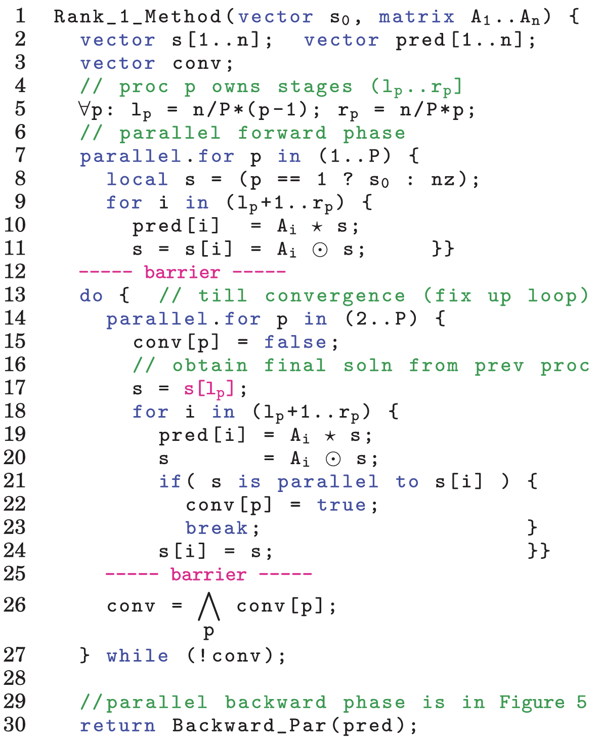
Fig. 4. The Rank-1 method for parallelizing the forward pass of LTDP that relies on rank-1 convergence for efficiency. All interprocessor communication is shown in magenta.

4.4. The Rank-1 Method: Parallelizing Forward Phase

The goal of the Rank-1 method in Figure 4 is to compute a solution vector s[i] at stage $i$ that is parallel to the actual solution vector $\bar{s}_i$ , as shown in Figure 3. During the execution of the algorithm, we say that a stage $i$ has converged if s[i] computed by the algorithm is parallel to its actual solution vector $\bar{s}_i$ .

The Rank-1 method splits the stages equally among $P$ processors such that a processor $p$ owns stages between $\mathbb{1}_{\mathbb{P}}$ (exclusive) and $\mathbb{r}_{\mathbb{P}}$ (inclusive), as shown in line 5. While processor 1 starts its computation from $\bar{s}_0$ , other processors start from some vector nz (line 8). This initial vector can be arbitrary, except none of its entries can be $\mathbb{O} = - \infty$ . Section 4.5 explains the importance of this constraint.

The loop starting in line 9 is similar to the sequential forward phase (Figure 2) except that the parallel version additionally stores the computed s[i] needed in the convergence loop in line 13.

Consider a processor $p \neq 1$ that owns stages ( $\mathbb{1}_{\mathbb{P}} = l \ldots r = \mathbb{r}_{\mathbb{P}}$ ). If there exists a stage $k$ in $(l \ldots r]$ such that rank $(M_{l \to k})$ is 1, then stage $k$ converges, irrespective of the initial vector nz (Lemma 2.2). Moreover, by Equation (3), rank $(M_{l \to j})$ is 1 for all stages $j$ in $[k \ldots r]$ , implying that these stages converge as well (Figure 3(b)). However, processor $p$ is not cognizant of the actual solution vectors and, thus, does not know the value of $k$ or whether such a $k$ exists.

The fix-up loop starting at line 13 (fix-up phase in Figure 3(c)) fixes stages $i < k$ . In this loop, processor $p$ receives the vector at stage $l$ computed by the previous processor $p - 1$ . (Figure 4 shows all such interprocessor communication in magenta.) Processor $p$ then updates s[i] for all stages till the new value becomes parallel to the old value of s[i] (line 21). This ensures that all stages owned by $p$ have converged, under the assumption that stage $l$ has converged.

In addition, the Boolean variable conv[p] indicates whether processor $p$ advertised a converged value for its last stage to processor $p + 1$ at the beginning of the iteration. Thus, when conv (line 26) is true, all stages have converged. In the ideal case, every processor has a partial product with rank 1, and thus, the fix-up loop executes exactly one iteration. Section 7 shows that we observe the best case for many practical instances.

Say, however, that conv[p] is not true for processor $p$ . This indicates that the stages $(1_p \ldots r_p]$ were not large enough to generate a partial product with rank 1. In the next iteration of the fix-up phase, processor $p + 1$ , in effect, searches for rank convergence in the wider range $(1_p \ldots r_{p+1}]$ . The fix-up loop iteratively combines the stages of the processors till all processors converge. In the worst case, the fix-up loop executes $P - 1$ iterations and the Rank-1 method devolves to the sequential case in Figure 2.

Important to note is that even though the previous discussion refers to partial products, the algorithm does not perform any matrix-matrix multiplications. Like the sequential algorithm, the presentation hides many implementation details in the $\star$ and $\odot$ operations (in lines 10, 11, 19, and 20). In fact, the Rank-1 method can reuse efficient implementations of these operations, including those that use wavefront parallelism, from existing sequential implementations. Also, the computation of conv at line 26 is a standard reduce operation that is easily parallelized, if needed.

When compared to the sequential algorithm in Figure 2, the Rank-1 method has to additionally store s[i] per stage required to test for convergence in the fix-up loop. If space is a constraint, then the fix-up loop can be modified to recompute s[i] in each iteration, trading compute for space.

4.5. All-Non-Zero Invariance

A subtle issue with the correctness of the previous algorithm is that starting the LTDP computation midway with an arbitrary initial vector nz could produce a zero vector (one with all $\mathbb{O} = -\infty$ entries) at some stage. If this happens, all subsequent stages will produce a zero vector, resulting in an erroneous result. To avoid this, we ensure that nz is all-non-zero; that is, none of its elements are $\mathbb{O} = -\infty$ .

A transformation matrix $A$ is nontrivial if every row of $A$ contains at least one nonzero entry. In Equation (1), the $j$ row of matrix $A_i$ captures how the subproblem $j$ in stage $i$ depends on the subproblems in stage $i - 1$ . If all entries in this row are $-\infty$ , then the subproblem $j$ is forced to be $-\infty$ for any solution to stage $i - 1$ . Such trivial subproblems can be removed from a given LTDP instance. So, we can safely assume that transformation matrices in LTDP instances are nontrivial.

LEMMA 4.1. For a nontrivial transformation matrix $A$, $$\vec{v}\text{ is all-non-zero} \Rightarrow A\odot \vec{v}\text{ is all-non-zero}.$$

$(A\odot \vec{v})[i] = \max_{k}(A[i,k] + \vec{v}[k])$ . But $A[i,k] \neq -\infty$ for some $k$ , ensuring that at least one of the arguments to max is not $-\infty$ . Here we rely on the fact that no element has an inverse under max, except $-\infty$ . As such, this lemma is not necessarily true in other semirings.

Thus, starting with an all-non-zero vector ensures that none of the stages results in a zero vector.

4.6. Parallel Backward Phase

Once the parallel forward phase is done, performing the sequential backward phase from Figure 2 will generate the right result, even though s[i] is not exactly the same as the correct solution $\vec{s}_i$ . In many applications, the forward phase overwhelmingly dominates the execution time, and parallelizing the backward phase is not necessary. If this is not the case, the backward phase can be parallelized using the same idea as the parallel forward phase as described later.

The backward phase recursively identifies the predecessor at stage $i$ starting from stage $n$ . One way to obtain this predecessor is by iteratively looking up the predecessor products pred[i] computed during the forward phase. Another way to obtain this is through repeated matrix multiplication as $M_{i \leftarrow n} \star \vec{s}_i$ , where $M_{i \leftarrow n}$ is the backward partial product $A_n \odot \ldots \odot A_{i+1}$ . Using the same rank convergence argument, the rank of $M_{i \leftarrow n}$ will converge to 1 for a large enough number of matrices (small enough $i$ ). Lemma 4.2 shows that the predecessor at stages beyond $i$ does not depend on the initial value used for the backward phase.

LEMMA 4.2. For a matrix A of rank 1 and any vector $\vec{v}$ , all elements of $A \star \vec{v}$ are equal.

This lemma follows from the fact that the rows in a rank-1 matrix only differ by a constant and $\arg \max$ is invariant when an offset is added to all its arguments.

The algorithm in Figure 5 uses this insight for a parallel backward phase. Every processor starts the predecessor traversal from 0 (line 8) on the stages it owns. Each processor enters a fix-up loop whose description and correctness mirror those of the forward phase discussed in Section 4.4.

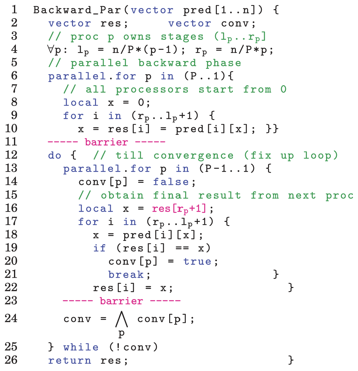
Fig. 5. Parallel algorithm for the backward phase of LTDP that relies on rank-1 convergence for efficiency. All interprocessor communication is shown in magenta.

4.7. Rank Convergence Discussion

One can view solving an LTDP problem as computing shortest/longest paths in a graph. In this graph, each subproblem is a node and directed edges represent the dependencies between subproblems. The weights on edges represent the constants $A_{i}[j,k]$ in Equation (1). In LCS, for instance (Figure 1), each subproblem has incoming edges with weight 0 from the subproblem above and to its left, and an incoming edge with weight $\delta_{i,j}$ from its diagonal neighbor. Finding the optimal solution to the LTDP problem amounts to finding the longest path in this graph from the subproblem 0 in the last stage to subproblems in the first stage, given initial weights to the latter. Alternately, one can negate all the weights and change the max to a min in Equation (1) to view this as computing shortest paths.

Entries in the partial product $M_{l\to r}$ represent the cost of the shortest (or longest) path from a node in stage $l$ to a node in stage $r$ . The rank of this product is 1 if these shortest paths go through a single node in some stage between $l$ and $r$ . Road networks have this property. For instance, the fastest path from any city in Washington State to any city in Massachusetts is highly likely to go through Interstate I-90 that connects the two states. Routes that use I-90 are overwhelmingly better than those that do not; choices of the cities at the beginning and at the end do not drastically change how intermediate stages are routed. Similarly, if problem instances have optimal solutions that are overwhelmingly better than other solutions, one should expect rank convergence.

5. THE PARALLEL DELTA METHOD

Section 3 describes sequential LTDP problems, and Section 4 introduces the parallel Rank-1 method, which relies on rank-1 convergence to be efficient. This section introduces the Delta method, an approach that relaxes the reliance on the rank-1 convergence for a subset of the LTDP problem.

The Delta method works for Local LTDP (LLTDP) problems. Figure 1(b) shows an example of an LLTDP where the dependencies for cell $C_{i,j}$ are the three local neighbors: $C_{i - 1,j}$ , $C_{i,j - 1}$ , and $C_{i - 1,j - 1}$ . In general, an LLTDP recursive function is given by

$$C_{i,j} = \max \left\{ \begin{array}{l}C_{i - 1,j} + w_{i,j}^{1}\\ C_{i,j - 1} + w_{i,j}^{2}\\ C_{i - 1,j - 1} + w_{i,j}^{3}, \end{array} \right. \quad (4)$$

where $w_{i,j}^{1}$ , $w_{i,j}^{2}$ , and $w_{i,j}^{3}$ are three constant terms that come from the inputs and are independent of the values of the cells. LLTDP problems are a subset of LTDP problems since Equation (4) restricts Equation (1)'s max terms to only the local neighbors (top, left, and top-left cells).

Figure 1(a) shows an LTDP example that is not local, and the dependencies for a cell come from all the cells of the previous stage. This structure of an LTDP problem prevents us from applying the Delta method, which we will discuss in Section 5.1.

5.1. The Delta Method

The intuition behind the Delta method is that instead of computing a value for each cell in an LLTDP problem, it computes the difference between local cells. For example, Figure 6(a) shows four cells: $C_{i - 1,j - 1}$ , $C_{i - 1,j}$ , $C_{i,j - 1}$ , $C_{i,j}$ . The Delta method computes $\delta_{i,j} = C_{i,j} - C_{i,j - 1}$ and $\Delta_{i,j} = C_{i,j} - C_{i,j - 1}$ instead of actually computing $C_{i,j}$ . Therefore, there are two delta values associated with each cell: the horizontal delta, $\delta$ , and the vertical delta, $\Delta$ . The whole computation only computes the deltas shown as red arrows in Figure 6(b). The key contribution of the Delta method is Lemma 5.1.

LEMMA 5.1. $\delta_{i,j}$ , $\Delta_{i,j}$ , and $\text{pred}_{i,j}$ can be computed given the values of $\delta_{i,j - 1}$ and $\Delta_{i - 1,j}$ and using recursive function 4.

PROOF. In Figure 6(a), assume that the value of $C_{i - 1,j - 1}$ is $x$ and, consequently, the values of $C_{i,j - 1}$ and $C_{i - 1,j}$ will be $x + \delta_{i - 1,j}$ and $x + \Delta_{i,j - 1}$ , respectively. Using the recursive function 4, $C_{i,j} = \max \{x + \delta_{i - 1,j} + w_{i,j}^{1},x + \Delta_{i,j - 1} + w_{i,j}^{2},x + w_{i,j}^{3}\}$ . Let $K = \max \{\delta_{i - 1,j} + w_{i,j}^{1},\Delta_{i,j - 1} + w_{i,j}^{2},w_{i,j}^{3}\}$ , and as a result, $C_{i,j} = x + K$ . $K$ is a constant since all of the terms are given. Therefore, $\delta_{i,j} = C_{i,j} - C_{i,j - 1} = x + K - (x + \Delta_{i,j - 1}) = K - \Delta_{i,j - 1}$ which is a constant. $\Delta_{i,j}$ can be similarly proven to be constant.

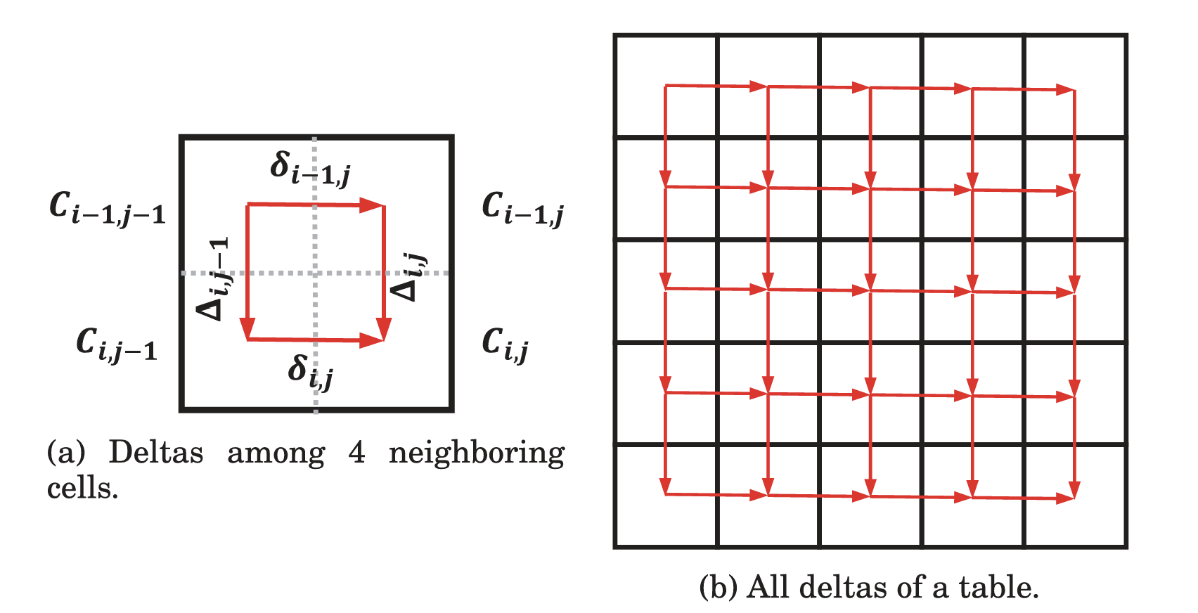
Fig. 6. The deltas among the cells.

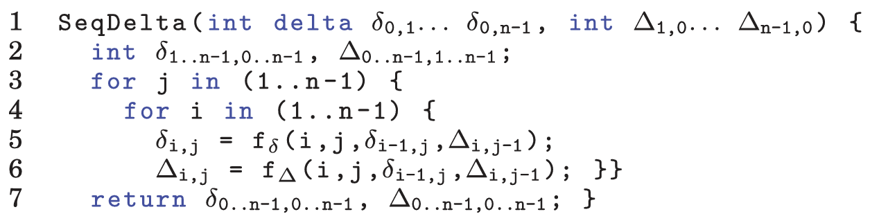
Fig. 7. The sequential Delta method for planar dynamic programming.

The arg max in the computation of $K$ is independent of $x$ and it corresponds to the same arg max in the computation of $C_{i,j}$ . Therefore, $pred_{i,j}$ is constant given the values of $\delta_{i,j - 1}$ and $\Delta_{i - 1,j}$ .

Figure 6(b) shows all deltas as red arrows in the table. Given all the initial deltas on the left and top side of the table, all other deltas can be computed using Lemma 5.1. Let $f_{\delta}(i,j,\delta_{i - 1,j},\Delta_{i,j - 1})$ and $f_{\Delta}(i,j,\delta_{i - 1,j},\Delta_{i,j - 1})$ be the functions that compute $\delta_{i,j}$ and $\Delta_{i,j}$ according to Lemma 5.1, respectively. Figure 7 shows the sequential algorithm for the Delta method. The inputs for the sequential Delta method are $\delta_{0,1},\ldots ,\delta_{0,n - 1},\Delta_{1,0},\ldots ,\Delta_{n - 1,0}$ , which are the initial deltas for the top and left side of the table. For the sake of simplicity, we assumed that the table is square shaped of size $n\times n$ . A lot of details are hidden behind the $f_{\delta}$ and $f_{\Delta}$ functions, which were described in detail in Lemma 5.1, including the computation of $pred_{i,j}$ values. We omitted them to reduce the complexity of the code. Note that we used type int for deltas, but the actual type depends on the type of values of $C$ in Equation (4). In certain cases, deltas have a smaller possible range of values, and as a consequence, more compact data types can be used to reduce memory and increase the efficiency in using SIMD units. Next, in Section 5.2, we will describe the parallel Delta method.

5.2. The Parallel Delta Method Overview

This section describes a parallel version of the Delta method, which is depicted in Figure 8. Figure 8(a) shows all deltas that are desired for computation. Assume that there are three processors available for the parallel computation: $P_{0}, P_{1},$ and $P_{2}$ . The set of deltas are distributed column-wise with one column of $\Delta s$ replicated at the boundaries, as shown in Figure 8(b). The parallel Delta method consists of two phases: (1) a random phase and (2) a fix-up phase. In the random phase, each processor except $P_{0}$ assumes random values for the first column of $\Delta s$ , as shown by dotted blue arrows in Figure 8(b) (Section 4.5 details how to pick random initial vectors). The key contribution of the parallel Delta method is the following observation.

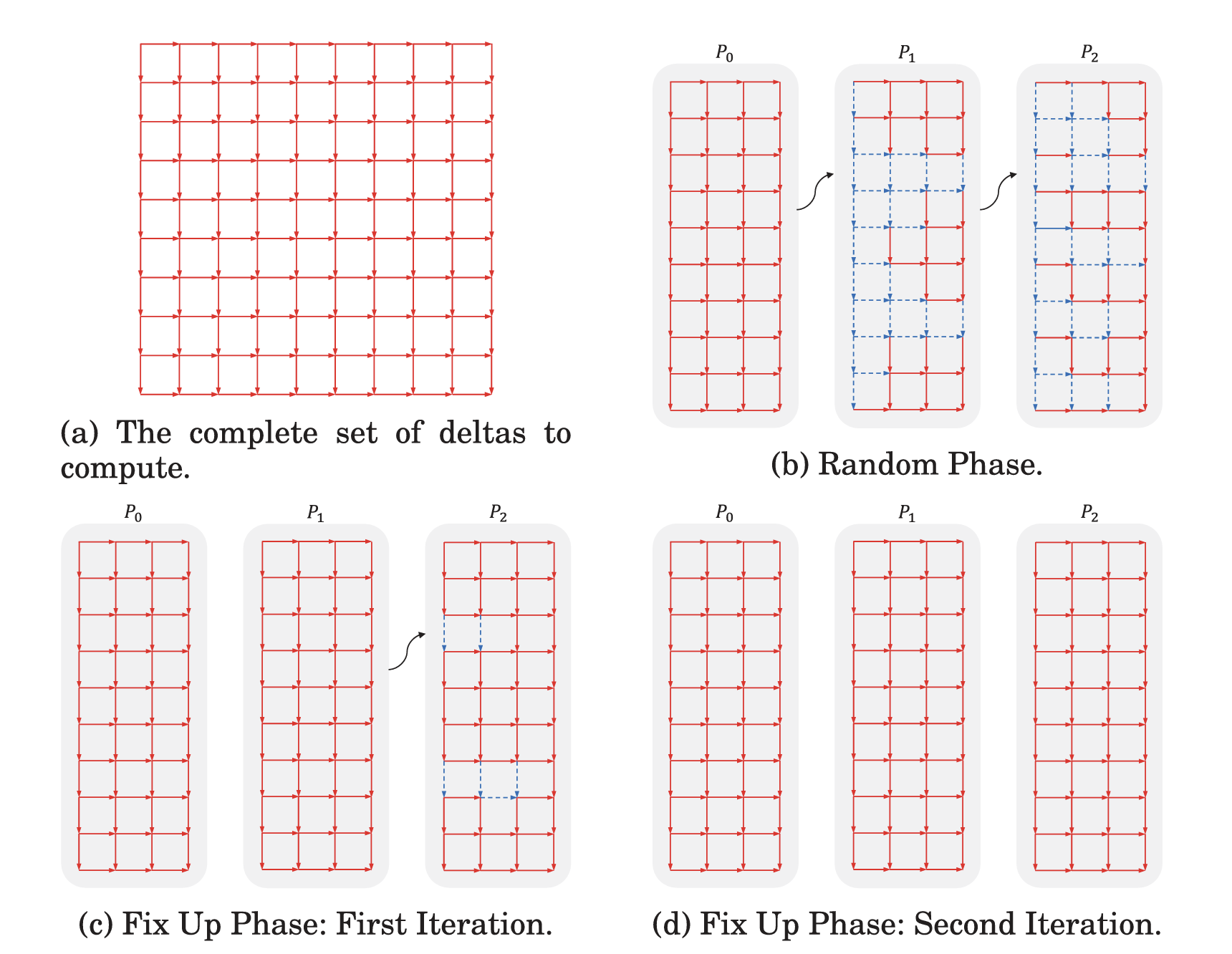
Fig. 8. The parallel Delta method. The solid red and dashed blue arrows represent the correct and wrong deltas, respectively. The first columns for $P_{1}$ and $P_{2}$ in (b) start with all dashed blue deltas since they are all picked randomly.

OBSERVATION 5.2. Starting with random (and perhaps incorrect) initial $\Delta s$ in the first column of a processor leads to many correct deltas on subsequent columns.

For cell $\{i,j\}$ , define input deltas to be $\delta_{i - 1,j}$ and $\Delta_{i,j - 1}$ and output deltas to be $\delta_{i,j}$ and $\Delta_{i,j}$ . This naming comes from Lemma 5.1, where, by taking the two input deltas, the two output deltas can be computed. As can be seen in Figure 8(b), starting with all incorrect random input deltas in the first column of $P_{1}$ and $P_{2}$ (shown as blue dotted arrows) leads to many correct output deltas (shown as red solid arrows) as the processors proceed. The deltas that are farther from the random initialization are more likely to be correct.

Denote predecessors and delta values that are computed using the random initialization by $pred_{i,j}^{\prime}$ , $\delta_{i,j}^{\prime}$ , $\Delta_{i,j}^{\prime}$ , and $C_{i,j}^{\prime}$ . The intuition behind Observation 5.2 is that $pred_{i,j} = pred_{i,j}^{\prime}$ for many cells. Assume that in Figure 6(a), both $\delta_{i - 1,j}^{\prime} \neq \delta_{i - 1,j}$ and $\Delta_{i,j - 1}^{\prime} \neq \Delta_{i,j - 1}$ , but $pred_{i,j} = pred_{i,j}^{\prime} = \{i - 1,j\}$ . Therefore, according to formula 4, $C_{i,j}^{\prime} = C_{i - 1,j}^{\prime} + w_{i,j}^{1}$ and similarly $C_{i,j} = C_{i - 1,j} + w_{i,j}^{1}$ , which means that $\Delta_{i,j}^{\prime} = w_{i,j}^{1} = \Delta_{i,j}$ . Hence, using incorrect input deltas may lead to correct output deltas. Also, correct deltas lead to more correct deltas because of Lemma 5.1.

The other observation that comes directly from Lemma 5.1 is that a blue dotted incorrect delta in Figure 8(b) has to come from another incorrect input delta. In other words, if there are two correct input deltas, the output deltas are also correct. Therefore, we can claim the following lemma.

LEMMA 5.3. If there is a path of solid red correct deltas from the top row of the table to the bottom of the table in a processor, the rest of the deltas after that path are solid red correct deltas.

PROOF. The top-row deltas are always correct since they are a part of initialization. Therefore, because of Lemma 5.1, all deltas that come immediately after the path are all correct. We can apply the same reasoning to conclude that the rest of the deltas after the path are all correct.

Using Observation 5.2 and Lemma 5.3, the rest of the parallel Delta method can be described. After each processor finishes its computation using a random initialization, $P_{i - 1}$ sends the last column of $\Delta s$ it owns to $P_{i}$ for $i = 1,2$ (as shown by black arrows in Figure 8(b)). This concludes the first phase of the parallel Delta method, which was called the random phase.

Next, the fix-up phase starts where the first iteration is depicted in Figure 8(c). In this phase, $P_{0}$ is idle while $P_{1}$ and $P_{2}$ fix up the incorrect deltas. Since each incorrect delta only affects its output deltas, each processor needs to recompute only $\delta_{i,j}$ s and $\Delta_{i,j}$ s, where $\delta_{i - 1,j}\neq \delta_{i - 1,j}^{\prime}$ or $\Delta_{i,j - 1}\neq \Delta_{i,j - 1}^{\prime}$ . Therefore, $P_{1}$ and $P_{2}$ perform less work in the first iteration of the fix-up phase than the random phase. At the end of the first iteration of the fix-up phase, only $P_{1}$ sends its correct deltas to $P_{2}$ . In the second iteration of the fix-up phase, $P_{0}$ and $P_{1}$ are both idle while $P_{2}$ fixes up the incorrect deltas, as shown in Figure 8(d). $P_{2}$ performs less work in the second iteration of the fix-up phase than the first iteration of the fix-up phase because there are fewer incorrect deltas after the first fix-up phase.

5.3. The Parallel Delta Method Implementation

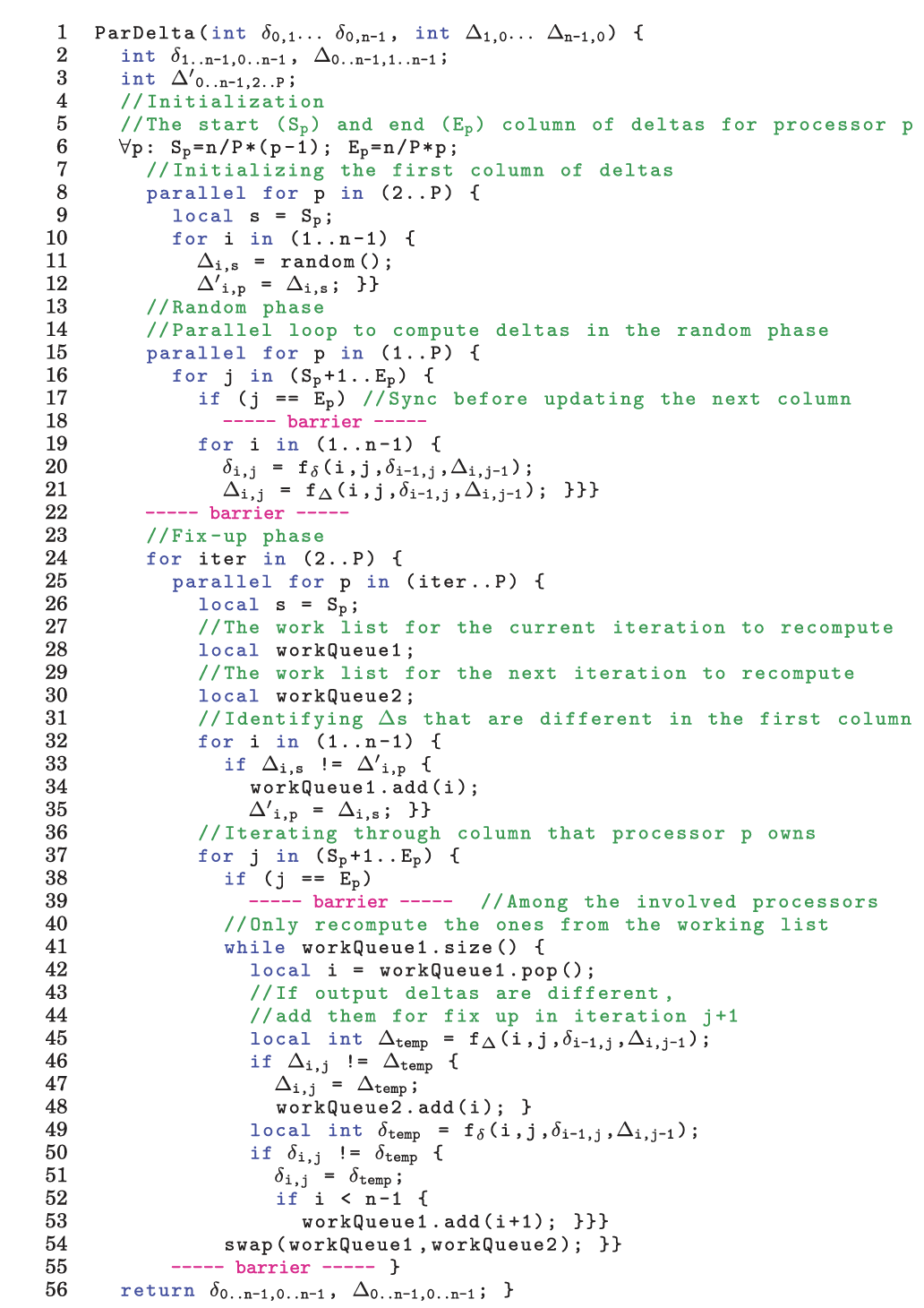
Fig. 9. The Parallel Delta method for LLTDP.

Figure 9 shows the parallel Delta method for LLTDP problems. First, we describe the initialization. The input arguments are given in line 1. Assume that there are $P$ processors available to the system. Then, each processor $p\in \{1\ldots P\}$ in line 6 computes the index for the first column and the last column of the range of deltas that it is assigned to, which are specified by $S_{p}$ and $E_{p}$ , respectively. Next, each processor $p$ , except the first one, initializes $\Delta s$ for column $s = S_{p}$ randomly in line 8. In line 12, the random $\Delta$ values for the first column of each processor are stored in $\Delta_{i,p}^{\prime}$ and are used later in the fix-up phase.

Next, in the random phase, each processor computes the deltas it owns in the loop in line 15. This loop is similar to the one from the sequential Delta method in Figure 7 except that it is parallel. In the final iteration of the loop in line 15, each processor $p$ updates the $\Delta s$ for the first column of processor $p + 1$ . Therefore, before this update, there is a barrier in line 18 to avoid data races. There is another barrier in line 22 after the parallel loop in line 15.

After the random phase, there is the fix-up phase and the main loop is in line 24. The first processor, $p_{1}$ , does not need the fix-up phase since all of its deltas are correct. $p_{2}$ needs one iteration of the fix-up phase since it receives the completely correct deltas after the random phase. $p_{3}$ needs at most two iterations of the fix-up phase since it eventually receives all correct deltas after the first iteration of the fix-up phase. In general, processor $p_{i}$ requires $i - 1$ iterations of the fix-up phase, which is specified by the range of the loop in line 25. The main fix-up loop in line 24 iterates for $P - 1$ times since the last processor may require $P - 1$ iterations of the fix-up phase.

For each processor in the fix-up phase, there are two work lists that keep track of the indices of incorrect delta inputs whose output deltas need to be recomputed: workQueue1 in line 28 and workQueue2 in line 30. They are used for different iterations of the loop in line 37 that goes through all columns of processor $p$ . workQueue1 is the work list for the current iteration of the loop $(j)$ , and workQueue2 is the work list for the next iteration of the loop $(j + 1)$ . Before the loop in line 37, the loop in line 32 initiates workQueue1 in line 33 by comparing the newly received $\Delta s$ and the $\Delta s$ used previously, which were saved in $\Delta 's$ in line 12. The ones that do not match are added in workQueue1 for recomputation of output deltas in line 34. Also, $\Delta '$ stores the new $\Delta s$ for the iteration of the fix-up phase in line 35.

The loop in line 37 goes through all columns of $p$ , and the while loop in line 41 goes through the workQueue1 and recomputes the necessary deltas. If a $\Delta$ for the next column is different from the previous iteration, it is added in workQueue2 in line 46 for the next iteration, $j + 1$ . On the other hand, if a $\delta$ is different, it affects the current iteration and the necessary index is added to workQueue1 in line 50. At the end, the two work lists are swapped in line 54 for the next iteration of the loop in line 37. Similar to the random phase, there is a necessary barrier in line 39 for the final iteration of the loop in line 37. The barrier in line 55 is the end of a fix-up iteration.

5.4. Algorithmic Comparison of the Parallel Delta Method and the Parallel Rank-1 Method

The parallel Rank-1 method in Section 4 can be explained using deltas for LLTDP. The parallel LTDP algorithm only relies on Lemma 5.3, and the fix-up phase is more coarse grained than the parallel Delta method. In the Rank-1 method, every processor similarly starts with a random initialization, but in the fix-up phase, all deltas for every column are recomputed until a column with all correct $\Delta s$ is reached. Because of Lemma 5.3, after such a column, the rest of the deltas are correct and there is no need for recomputation.

The new parallel Delta method approach recomputes only a subset of the deltas in a column where that subset is identified using Lemma 5.1. Therefore, the parallel Delta method is an improvement to the Rank-1 method and the expectation is that the Delta method is never slower than the Rank-1 method for LLTDP problems. Specially in the cases where it takes a lot of columns to converge to rank 1, the Delta method should be significantly faster. Section 7 studies this comparison in practice.

6. LTDP EXAMPLES

This section shows four important optimization problems as LTDP: Viterbi, Longest Common Subsequence, Smith-Waterman, and Needleman-Wunsch. Our goal in choosing these particular problems is to provide an intuition on how problems with different structures can be viewed as LTDP. Other problems that are LTDP but not evaluated in this article include dynamic time warping and seam carving.

Viterbi. The Viterbi algorithm [Viterbi 1967] finds the most likely sequence of states in a (discrete) hidden Markov model (HMM) for a given sequence of $n$ observations. Its recurrence equation is shown in Figure 1(a). Here, $p_{i,j}$ represents the probability of the most likely state sequence ending in state $j$ of the HMM that explains the first $i$ observations. The meaning of the term $t_{k,j}$ is not important here (see Viterbi [1967]). The solution to a Viterbi instance is given by the maximum value of $p_{n,j}$ as we are interested in the most likely sequence ending in any HMM state.

The subproblems along a column in Figure 1(a) form a stage, and they only depend on the subproblems in the previous column. This dependence is not directly in the desired form of Equation (1). But applying a logarithm on both sides to the recurrence equation brings it to this form. By transforming the Viterbi instance into one that calculates log-probabilities instead of probabilities, we obtain an LTDP instance.

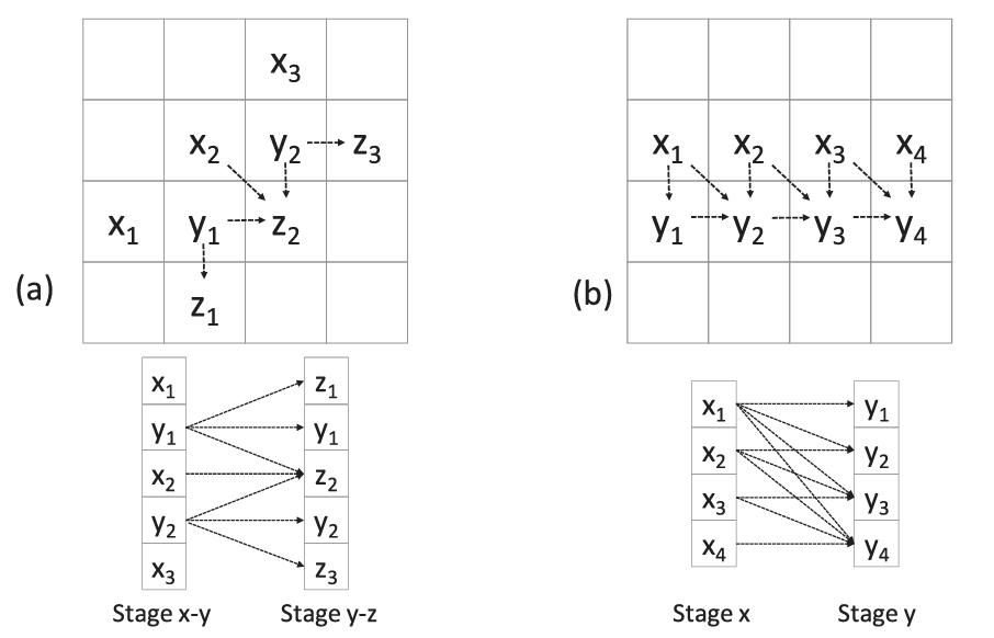
Fig. 10. Two ways of grouping the subproblems in LCS into stages such that each stage only depends on one previous stage.

Invoking the LTDP parallel algorithm in Figure 4 requires one additional transformation. The algorithm assumes that the solution to LTDP is given by the first subproblem in the last stage $n$ . To account for this, we introduce an additional stage $n + 1$ in which every subproblem is the maximum of all subproblems in stage $n$ . Essentially, stage $n + 1$ is obtained from multiplying a matrix with 0 in all entries with stage $n$ .

The Viterbi algorithm is not an LLTDP since the dependence edges are not local and they cross. Therefore, the Delta method is not applicable.

Longest Common Subsequence. LCS finds the longest common subsequence of two input strings $A$ and $B$ [Hirschberg 1975]. The recurrence equation of LCS is shown in Figure 1(b). Here, $C_{i,j}$ is the length of the longest common subsequence of the first $i$ characters of $A$ and the first $j$ characters of $B$ . Also, $\delta_{i,j}$ is 1 if the $i$th character of $A$ is the same as the $j$th character of $B$ and 0 otherwise. The LCS of $A$ and $B$ is obtained by following the predecessors from the bottom-rightmost entry in the table in Figure 1(b).

Some applications of LCS, such as the diff utility tool, are only interested in solutions that are at most a width $w$ away from main diagonal-ensuring that the LCS is still reasonably similar to the input strings. For these applications, the recurrence relation can be modified such that $C_{i,j}$ is set to $-\infty$ whenever $|i - j| > w$ . Using a smaller width also reduces the memory requirements of LTDP as the entire table need not be stored in memory. Smaller width limits the scope of wavefront parallelism due to smaller sizes of stages, which emphasizes the need for parallelizing across stages as proposed by this article.

LCS is an LLTDP problem as it can be checked from Figure 10. Therefore, the parallel Delta method from Section 5.2 can be applied, although using this method instead of the Rank-1 method requires computing two values per cell. One can show that deltas in the LCS problem are either 1 or 0. This allows compactly representing the deltas as a sequence of bits [Hyyro 2004]).

On the other hand, LCS is also an LTDP problem, and the Rank-1 method requires defining stages such that a stage is only dependent on the previous stage. Grouping the subproblems of LCS into stages can be done in two ways, as shown in Figure 10. In the first approach, the stages correspond to antidiagonals, such as the stage consisting of $z_{1}$ s in Figure 10(a). This stage depends on two previous stages (on $x_{1}$ s and $y_{1}$ s) and does not strictly follow the rules of LTDP. One way to get around this is to define stages as overlapping pairs of antidiagonals, like stage $x - y$ and stage $y - z$ in Figure 10(a). Subproblems $y_{1}$ s are replicated in both stages, allowing stage $y - z$ to depend only on stage $x - y$ .

In the second approach, the stages correspond to the rows (or columns) as shown in Figure 10(b). The recurrence needs to be unrolled to avoid dependencies between subproblems within a stage. For instance, $y_{1}$ depends on all $x_{j}$ for $j \leq i$ . In this approach, since the final solution is obtained from the last entry, the predecessor traversal in Figure 2 has to be modified to start from this entry, say, by adding an additional matrix at the end to move this solution to the first solution in the added stage.

Needleman-Wunsch. This algorithm [Needleman and Wunsch 1970] finds a global alignment of two input sequences, commonly used to align protein or DNA sequences. The recurrence equation is very similar to the one in LCS (Section 6):

$$s_{i,j} = \max \begin{cases} s_{i-1,j-1} + m[i, j] \\ s_{i-1,j} - d \\ s_{i,j-1} - d. \end{cases}$$

In this equation, $s_{i,j}$ is the score of the best alignment for the prefix of length $i$ of the first input and the prefix of length $j$ of the second input, $m[i,j]$ is the matching score for aligning the last characters of the respective prefixes, and $d$ is the penalty for an insertion or deletion during alignment. The base cases are defined as $s_{i,0} = - i * d$ and $s_{0,j} = - j * d$ .

The Needleman-Wunsch algorithm is also an LLTDP problem as it can be checked from the formula. Therefore, as in the LCS case, the Delta method is applicable to this algorithm. Similarly, one can show that deltas are in the range of $[- d \ldots (\max_{i,j} m[i,j] + d)]$ , allowing compact representation.

To apply the Rank-1 method, subproblems can be grouped into stages using the same approach as in LCS. Abstractly, one can think of LCS as an instance of Needleman-Wunsch for appropriate values of matching scores and insert/delete penalties. However, the implementation details differ sufficiently enough for us to consider them as two different algorithms.

Smith-Waterman. This algorithm [Smith and Waterman 1981] performs a local sequence alignment, in contrast to Needleman-Wunsch. Given two input strings, Smith-Waterman finds the substrings of the input that have the best alignment, where longer substrings have a better alignment. In its simplest form, the recurrence equation is of the form

$$s_{i,j} = \max \begin{cases} 0 \\ s_{i-1,j-1} + m[i, j] \\ s_{i-1,j} - d \\ s_{i,j-1} - d. \end{cases}$$

The key difference from Needleman-Wunsch is the 0 term in max, which ensures that alignments "restart" whenever the score goes to zero. Because of this term, the constants in $A_{i}$ matrices in Equation (1) need to be set accordingly. This slight change has a significant difference from the convergence properties of Smith-Waterman as we will see later in Section 7.1. Our implementation uses a more complex recurrence equation that allows for affine gap penalties when aligning sequences [Farrar 2007].

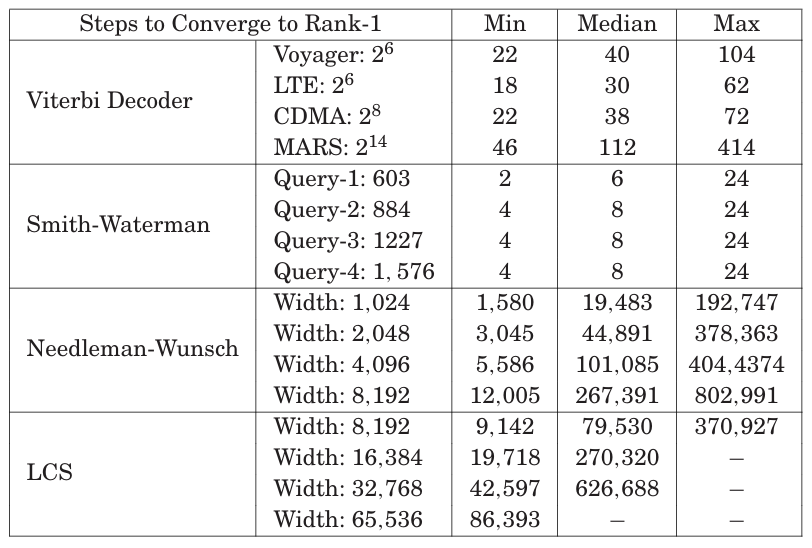
Table I. Number of Steps to Converge to Rank 1

Also, the solution to Smith-Waterman requires finding the maximum of all subproblems in all stages and performing a predecessor traversal from that subproblem. To account for this in our LTDP formulation, we add one "running maximum" subproblem per stage that contains the maximum of all subproblems in the current stage and previous stages.

The Smith-Waterman algorithm is not an LLTDP, and therefore, the parallel Delta method is not applicable.

7. EVALUATION

This section evaluates the parallel LTDP algorithm on the four problems discussed in Section 6. Section 7.1 empirically evaluates the occurrence of rank convergence in practice. Section 7.2 describes the environmental setup. Section 7.3 evaluates the scalability, speedup, and efficiency of our implementation. Section 7.4 compares the performance of the Delta method with the Rank-1 method for LLTDP problems. Finally, Section 7.5 compares the parallel methods with wavefront parallelization.

7.1. LTDP Rank Convergence

Determining whether the LTDP parallel methods benefit a dynamic programming problem requires (1) the problem to be LTDP (discussed in Section 3) and (2) rank convergence to happen in a reasonable number of steps. This section demonstrates how rank convergence can be measured and evaluates it for the four LTDP problems discussed in Section 6.

Rank convergence is an empirical property of a sequence of matrix multiplications that depends on both the LTDP recurrence relation and the input. Table I empirically evaluates the number of steps required for the rank-1 convergence across different algorithms and inputs. For an LTDP instance, defined by the algorithm (Column 1) and input (Column 2), we first compute the actual solution vectors at each stage. Then, starting from a random all-non-zero vector at 200 different stages, we measured the number of steps required to generate a vector parallel to the actual solution vector (i.e., convergence). Columns 3, 4, and 5 respectively show the minimum, median, and maximum number of steps needed for convergence. For each input, Column 2 specifies the computation width (the size of a stage or the size of each $A_{i}$ matrix). Each algorithm has a specific definition of width: for the Viterbi decoder, width is the number of states for each decoder; in Smith-Waterman, it is the size of each query; and in LCS and Needleman-Wunsch, it is a fixed width around the diagonal of each stage. The missing entries for LCS mean the convergence never happened. The rate of convergence is specific to the algorithm and input (i.e., Smith-Waterman converges fast while LCS sometimes does not converge), and, generally speaking, wider widths require more steps to converge. We will use this table later in Section 7.3 to explain the scalability of our approach.

Table II. Algorithms Used for Each LTDP Problem

7.2. Environmental Setup

We conducted experiments on a shared-memory machine and on a distributed-memory machine. A shared-memory machine favors fast communication and is ideal for the wavefront approach. Likewise, a distributed machine has a larger number of processors and so we can better understand how our parallel algorithm scales. Next, we describe these two machines.

Distributed-Memory Machine. Stampede [Texas Advanced Computing Center Texas Advanced Computing Center], a Dell PowerEdge C8220 Cluster with 6,400 nodes. At the time of writing this article, Stampede is ranked sixth on the Top500 [Top500 Supercompute Sites 2013] list. Each node contains two 8-core Intel Xeon E5-2600 processors $@2.70\mathrm{GHz}$ (16 cores in total) and 32GB of memory. The interconnect topology is a fat-tree, FDR InfiniBand interconnect. On this cluster, we used the MPI MVAPICH 2 library [MVAPICH: MPI over InfiniBand 2013] and the Intel C/C++ compiler version 13.0.1 [Intel C/C++ Compiler 2013]. We never used more than 128 cores on this machine for our experiments.

Shared-Memory Machine. An unloaded Intel 2.27GHz Xeon (E7) workstation with 40 cores (80 threads with hyperthreading) and 128GB RAM. We use the Intel C/C++ compiler (version 13.0.1) [Intel C/C++ Compiler 2013] and the Intel MPI library (version 4.1) [Intel MPI Library 2013].

We report scalability results on Stampede, but results from the shared-memory machine are qualitatively similar. We used the shared-memory machine to compare our parallel algorithm with wavefront parallelization. Unless specified otherwise, the reported results are from Stampede runs.

We use the MPI/OMP timer to measure process runtime. We do not measure setup costs-only the time it takes to execute one invocation of an LTDP problem. When we compare against a baseline, we modify that code to take the same measurements.

Finally, to get statistically significant results, we run each experiment multiple times and report the mean and $95\%$ confidence interval of the mean when appropriate. We do not include confidence intervals in the graphs if they are small.

7.3. LTDP Benchmarks and Performance

This section evaluates the parallel methods on the four LTDP problems discussed in Section 6. Table II lists what algorithms are used for baseline and parallelization of each LTDP problem. We will discuss each of them in detail in this section.

To substantiate our scalability results, we evaluate each benchmark across a wide variety of real-world inputs. We break the results down by the LTDP problem.

7.3.1. Viterbi Decoder.

The Viterbi decoder uses the Viterbi algorithm (Section 6) to communicate over noisy and unreliable channels, such as cell phone communications [Viterbi 1967]. Given a potentially corrupted convolution-encoded message [Peterson and Weldon 1972], Viterbi decoding finds the most likely unencoded message.

Baseline. We used Spiral's [Puschel et al. 2005] Viterbi decoder: a highly optimized (via autotuning) decoder that utilizes SIMD to parallelize decoding within a stage. To the best of our knowledge, there is no efficient multiprocessor algorithm for Viterbi decoders since the amount of parallelism in each stage is limited.

Our Implementation. Spiral code is heavily optimized, and even small changes negatively affect performance. Therefore, the performance-critical internal loop of the Spiral code is used as a black box. Viterbi is not LLTDP and therefore we only implemented the Rank-1 method. Each processor starts from an arbitrary all-non-zero vector (except the first, which uses the initial vector) and uses Spiral to execute its set of stages. Each processor (except the last) then communicates its result to the next processor.

Data. We use four real-world convolution codes: Voyager, the convolution codes used on NASA's deep space Voyager; Mars, the convolution codes used to communicate with NASA's Mars rovers; and both CDMA and LTE, two convolution codes commonly used in modern cell phone networks. For each of these four convolution codes, we investigate the impact of four network packet sizes (2,048, 4,096, 8,192, and 16,384), which determine the number of stages in the computation. For each size, we used Spiral's input generator to create 50 network packets.

Performance and Scalability. Figure 11 shows the performance, speedup, and efficiency of each of the four decoders. To evaluate the impact of different decoder sizes, each plot has four lines (one per network packet size). A point $(x,y)$ in a performance/speedup plot with the primary y-axis on the left gives the throughput $y$ (the number of bits processed in a second) in megabits per second (Mb/S) as a function of the number of processors $x$ used to perform the Viterbi decoding. The same point with the secondary y-axis on the right shows the speedup $y$ with $x$ number of processors over the sequential performance. Note that Spiral sequential performance at $x = 1$ is almost the same for different packet sizes. The filled data points in the plots show that convergence occurred in the first iteration of the fix-up loop in the Figure 4 algorithm (i.e., each processor's stage is large enough for convergence). The nonfilled data points show that multiple iterations of the fix-up loop were required. Similarly, a point in an efficiency plot provides the speedup of our parallel implementation over the sequential performance of Spiral-generated code divided by the number of processors. Each point is the mean of 50 random packets.

Figure 11 demonstrates that (1) our Rank-1 method provides significant speedups over the sequential baseline and (2) different convolution codes and network packet sizes have different performance characteristics. For example, with 64 processors, our CDMA Viterbi decoder processing packets of size 16,384 decodes at a rate of 434Mb/S, which is $24 \times$ faster than the sequential algorithm. Note that for the same network packet size and number of processors, our MARS decoder only processes at 4.4Mb/S because the amount of computations per bit (size of each stage) is significantly greater than CDMA.

The performance of our Rank-1 method-and thus our speedup numbers-depends on the rate of rank convergence for each pair of convolution codes and network size, as shown in Table I. A larger network packet size provides better performance across all convolution codes (i.e., a network packet size of 16,384 is always the fastest implementation, regardless of convolution code) because the amount of recomputation (i.e., the part of the computation that has not converged), as a proportion of the overall computation, decreases with a larger network packet size.

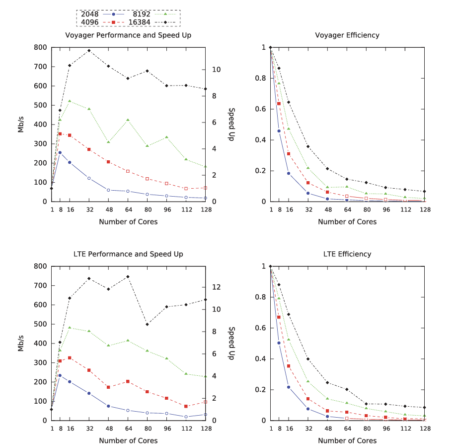
Fig. 11. Performance (Mb/S), speedup, and efficiency of Voyager and LTE Viterbi decoders with the parallel Rank-1 method. The nonfilled data points demonstrate where processors have too few iterations to converge to rank 1.

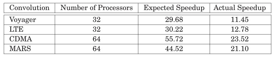
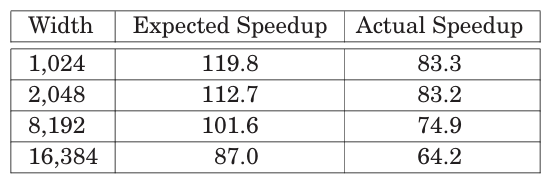
Table III. Comparison of the Expected Speedup and the Actual Speedup for Viterbi Decoder for Messages with Length 16,384

Also, as can be seen in Figure 11, efficiency plots drop as the packet sizes decrease and this is again because the ratio of the amount of recomputation to the whole computation decreases. Note that with 48 processors, our algorithm for CDMA can reach efficiency of more than 0.4.

Table III compares the actual speedup with the expected speedup. The expected speedup is computed by

$$\frac{w.l}{\frac{w.l}{P} + w.o},$$

where $w$ is the amount of computation per column, $l$ is the length of computation (packet size), $P$ is the total number of processors, and $o$ is the median number of steps for convergence to rank 1 taken from Table I. Essentially, $w.l$ is the total amount of work, $\frac{w.l}{l}$ is the amount of work per processor, and $w.o$ is the amount of work overhead for each processor. Therefore, the expected speedup is the theoretical speedup according to Amdahl's law. In Table III, only $l = 16,384$ is considered and the number of processors is chosen by the point where the Rank-1 method performs the best with this $l$ and the corresponding convolution code. As can be seen, there is a large difference between the expected and the real speedups, which means that the communication overhead is significant in this LTDP problem. This is not surprising since the amount of computation is very limited in this problem.

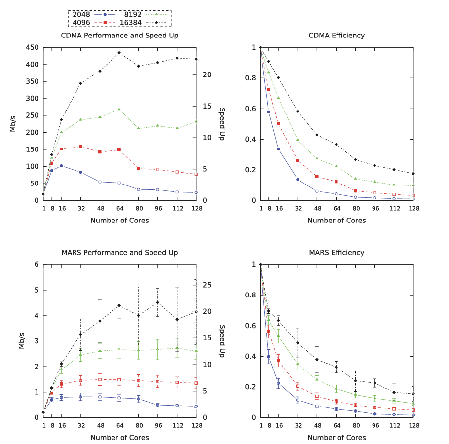
Fig. 12. Performance (Mb/S), speedup, and efficiency of CDMA and MARS Viterbi decoders with the parallel Rank-1 method. The nonfilled data points demonstrates where processors have too few iterations to converge to rank 1.

7.3.2. Smith-Waterman.

As described in Section 6, Smith-Waterman is an algorithm for local sequence alignment [Smith and Waterman 1981] often used to align DNA/protein sequences.

Baseline. We implemented the fastest known CPU version, Farrar's algorithm, which utilizes SIMD to parallelize within a stage [Farrar 2007].

Our Implementation. Smith-Waterman is not an LLTDP problem and we implemented the Rank-1 method using Farrar's algorithm as a black box.

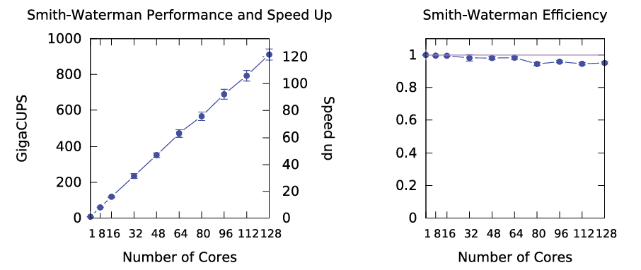
Fig. 13. Smith-Waterman performance, speedup, and efficiency.

Data. We aligned chromosomes 1, 2, 3, and 4 from the human reference genome hg19 as databases and four randomly selected expressed sequence tags as queries. All the inputs are publicly available to download from the National Center for Biotechnology Information [2013]. We report the average of performance across all combinations of DNA and queries (16 in total).

Performance and Scalability. A point $(x,y)$ in the performance/speedup plot in Figure 13 with the primary y-axis on the left gives the performance $y$ in Giga cell updates per second, or GigaCUPS, as a function of the number of processors used to perform the Smith-Waterman alignment. GigaCUPS is a standard metric used in bioinformatics to measure the performance of DNA-based sequence alignment problems and refers to the number of cells (in a dynamic programming table) updated per second. Similar to the Viterbi decoder plots, the secondary y-axis on the left shows the speedup for each number of processors. We run Smith-Waterman on all combinations of four DNA databases and four DNA queries (we run each combination 5 times). Unlike the prior Viterbi results, we do not see large variability in performance as a function of the problem data. In other words, the DNA database and query pairs do not significantly impact our performance numbers. This can also be confirmed from Table I, where the number of steps to converge to rank 1 is significantly smaller than a DNA database size that is more than 100 million characters long. Thus, we plot the average across all combinations of DNA databases and queries.

The performance gain of our approach for this algorithm is significant: the efficiency plot in Figure 13 demonstrates that our approach has efficiency $\sim 1$ for any number of processors, which means almost a linear speed-up with up to 128 processors. This can also be confirmed from the performance/speedup plot. Our algorithm would scale more with a larger number of processors, but we only report up to 128 processors to keep Figure 13 consistent with the others. Also, since the length of computation is significantly larger than the number of steps for convergence to rank 1 (100 million vs. 24), the expected speedup (explained earlier) is very close to the linear speedup. Therefore, we omitted the comparison between the expected and the actual speedup.

7.3.3. Needleman-Wunsch.

In contrast to Smith-Waterman, which performs a local alignment between two sequences, Needleman-Wunsch globally aligns two sequences and is often used in bioinformatics to align protein or DNA sequences [Needleman and Wunsch 1970].

Baseline. We utilized SIMD parallelization of the Delta method discussed in Section 5.1 within a stage for this benchmark. In other words, consecutive input deltas that are independent in a stage are used to compute output deltas for the next stage. Although computing deltas instead of the cell values requires more work (2 deltas per cell), the smaller range of possible values for deltas (as described in Section 6) enables the algorithm to use smaller data types for deltas and, consequently, fits more deltas in a single SIMD vector unit. Our experiments show that the Delta method is faster than computing cell values.

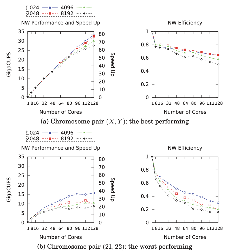
Fig. 14. Performance, speedup, and efficiency results of Needleman-Wunsch.

Our Implementation. We implemented the parallel Delta method described in Section 5.2.

Data. We used four pairs of DNA sequences as inputs: human chromosomes (17, 18), (19, 20), (21, 22), and $(X,Y)$ from the human reference genome hg19. We only used the first 1 million elements of the sequences since Stampede does not have enough memory on a single node to store the cell values for the complete chromosomes. We also tried four different width sizes: 1, 024, 2, 048, 4, 096, and 8, 192, since we found that widths larger than 8, 192 do not affect the final alignment score.

Performance and Scalability. Figure 14 shows the performance, speedup, and efficiency of the Needleman-Wunsch algorithm parallelized using the Delta method for two pairs of chromosomes: $(X,Y)$ and (21, 22). Instead of averaging performance numbers over all four pairs, we separated them and reported the best-performing pair $((X,Y)$ in Figure 14(a)) and the worst-performing pair ((21, 22) in Figure 14(b)). This is because the performance varies significantly between different pairs, as can be seen in Figures 14(a) and 14(b). The figures show results for each of the width sizes: 1, 024, 2, 048, 4, 096, and 8, 192. Similar to the Viterbi decoder benchmark, filled/nonfilled data points show whether convergence occurred in the first iteration of the fix-up phase.

Table IV. Comparison of the Expected Speedup and the Actual Speedup for Needleman-Wunsch Problem with 128 Processors

The figures show great variability in performance for different inputs based on the variability in convergence. Also, as can be seen from nonfilled data points and Table I, rank convergence in this benchmark is not as fast as in the Viterbi decoder or Smith-Waterman.

In Figure 14, larger widths perform more poorly than smaller ones since the convergence rate depends on the size of each stage in an LTDP instance. Note that we used the same sequence size (1 million element) for all plots.

Table IV compares the expected speedup and the actual speedup. For this LTDP problem, we measured the work overhead exactly and computed the expected speedup based on that. All numbers in Table IV are with 128 processors and for the alignment of the chromosomes $(X,Y)$ . As can be seen, the expected and the actual speedups are fairly close, unlike the Viterbi decoder. This means that the cost of communication in this problem is relatively small. This is, in fact, because only a few sets of values of size width are communicated, which is insignificant with respect to the whole computation (maximum width size is 16,384 but the computation is of size $16,384 \times 1,000,000$ ).

7.3.4. LCS.

Longest Common Subsequence is a method to find the largest subsequence common to two candidate sequences [Hirschberg 1975] (see Section 6 for description).

Baseline. We adapted the fastest-known single-core algorithm for LCS that exploits bit-parallelism to parallelize the computation within a row [Deorowicz 2010; Hyyro 2004]. This approach is similar to the Delta method from Section 5.1 and uses the grouping technique shown in Figure 10(b) but only computes the horizontal deltas.

Our Implementation. Similar to Needleman-Wunsch, we implemented the parallel Delta method described in Section 5.2 using the bit-parallel baseline code.

Data. We used the same input data as with Needleman-Wunsch except that we used the following width range: 8, 192, 16, 384, 32, 768, and 65, 536. We report performance numbers in the same way as in Needleman-Wunsch.

Performance and Scalability. The performance, speedup, and efficiency plots in Figure 15 are very similar to Figure 14. We used the same two pairs of chromosomes, $(X,Y)$ and (21, 22), as they are the best- and worst-performing pairs, respectively. The four lines in each plot correspond to one of the following width sizes: 8, 192, 16, 384, 32, 768, and 65, 536. Likewise, the input pair has a great impact on rank convergence, as can be seen in Figures 15(a) and 15(b).

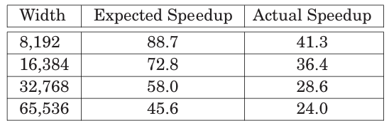
Table V compares the expected and the actual speedups. Similar to Needleman-Wunsch, we measured the work overhead exactly for this problem. All numbers in Table IV are with 128 processors and for the alignment of the chromosomes $(X,Y)$ . As can be seen, there is a large difference between the expected and the actual speedups. This is because of the communication overhead.

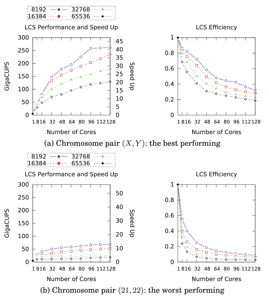
Fig. 15. Performance, speedup, and efficiency results of Longest Common Subsequence.

Table V. Comparison of the Expected Speedup and the Actual Speedup for Longest Common Subsequence Problem with 128 Processors

7.4. The Rank-1 Method Versus the Delta Method

This section shows the effectiveness of the Delta method compared to the Rank-1 method. For this purpose, we will compare the amount of extra work each algorithm performs along with the timings.

The Comparison for LCS. Figure 16 compares the two methods: the left plot shows the performance of the Delta method over the Rank-1 method for a different number of cores using different widths. The right plot shows the ratio of the total amount of work done in the last processor by the Rank-1 method to that done by the Delta method. We used the amount of work for the last processor because it needs the most iterations of the fix-up phase and, consequently, does the most work among all. As can be seen, the

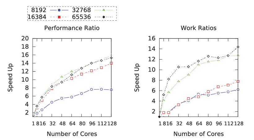
Fig. 16. The speedup of the Delta method over the Rank-1 method using LCS example.

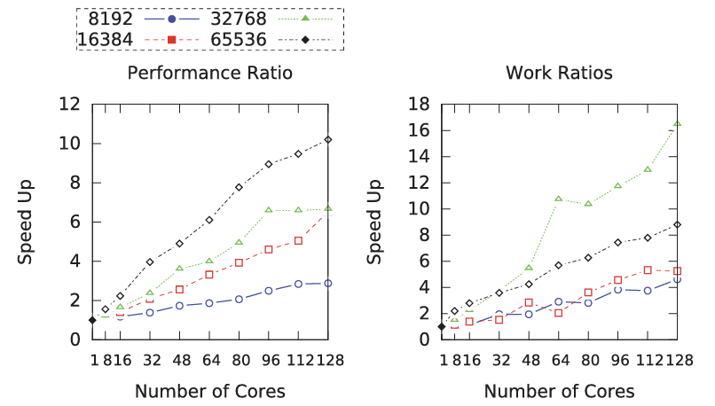
Delta method is between $\sim 5\times$ and $\sim 15\times$ faster than the Rank-1 method with 128 cores, which is compatible with the ratio of the amount of work for the last processor. Also, as can be expected, the Delta method has a greater impact with wider widths since the Rank-1 method recomputes all deltas even if only one of them is incorrect.

The Comparison for Needleman-Wunsch. Figure 17 similarly compares the two methods for the Needleman-Wunsch algorithm, and the plots show the performance speedup and the last processor work ratio. As can be seen, the Delta method is between $\sim 2\times$ and $\sim 10\times$ faster than the Rank-1 method with 128 cores. This again proves the effectiveness of the Delta method.

7.5. Wavefront Versus LTDP

Our goal in this section is to directly compare across-stage parallelism with wavefront parallelism. We focus on Needleman-Wunsch and LCS as the size of the stages in Viterbi and Smith-Waterman is very small for wavefront parallelism to be viable. We should note that the two approaches are complementary. Exploring the optimal way to distribute a given budget of processors to simultaneously use across-stage parallelism and within-stage parallelism is left for future work. Furthermore, note that we implemented the best-known wavefront algorithm for each of our benchmarks.

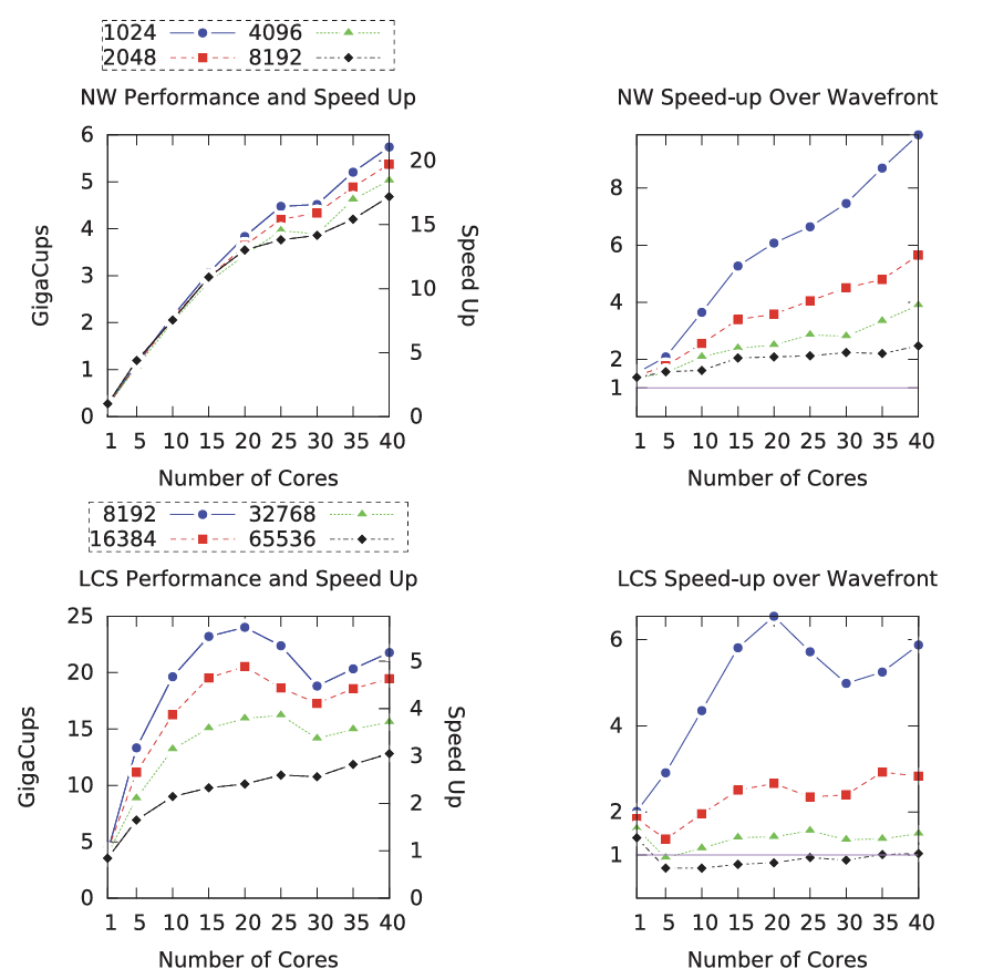
Fig. 18. Performance/speedup results and comparison of LTDP and wavefront for Needleman-Wunsch and LCS.

We used OpenMP for wavefront implementations and compared it with our MPI implementation used in our Stampede experiments earlier, but running on our shared-memory machine. This difference in implementation choice should at the worst bias the results against our parallel algorithm.

Wavefront for Needleman-Wunsch. We used tiling to group cells of the computation table and used SIMD in each tile. Wavefronts proceed along the antidiagonal of these tiles. Tiling greatly reduces the number of barriers involved [Martins et al. 2001]. On the other hand, processing cells in a tile by utilizing SIMD has computation overhead over the baseline that we used for our parallel approach (without tiling). Therefore, the sequential performance of the baseline with tiling is slower than the baseline without tiling. We investigated different tiling parameters and chose the best-performing configuration.

Wavefront for LCS. Similar to the baseline of Needleman-Wunsch, we tiled the cells. For computation in each cell, we used the same bit-parallelism to parallelize the computation within a column of each tile. Likewise, we parallelized computation of tiles that are in the same antidiagonal.

Figure 18 compares the performance of our approach with an optimized wavefront-based approach for both LCS and Needleman-Wunsch. The plots on the left in Figure 18 show the performance and speedup (over sequential nontiled baseline) of our approach for Needleman-Wunsch and LCS. In the plots on the right, a point $(x, y)$ gives the speedup $(y$ as runtime of wavefront divided by runtime of our approach) as we

change the number of processors allocated to each approach $(x)$ . We plot four lines, one for each of four widths. Small widths are better for our approach (as the wavefront approach incurs more barriers per unit of compute), while large widths are better for the wavefront approach (as our approach is less likely to reach rank 1). As we add more processors, our approach utilizes each additional processor more efficiently than a wavefront-based approach, particularly when the width is small (i.e., our approach is $\sim 9 \times$ faster than the wavefront approach with 40 processors for Needleman-Wunsch and $\sim 6 \times$ faster than the wavefront approach for LCS with width size 8,192).

8. RELATED WORK

An earlier version of this article was published in Maleki et al. [2014], where only the Rank-1 method was studied. This article introduces the Delta method, which is an improvement over the Rank-1 method.

There has been a lot of prior work in parallelizing dynamic programming. Predominantly, implementations use wavefront parallelism to parallelize within a stage. In contrast, this article exploits parallelism across stages in addition to wavefront parallelism. For instance, Martins et al. [2001] build a message-passing-based implementation of sequence alignment dynamic programs (i.e., Smith-Waterman and Needleman-Wunsch) using wavefront parallelism. Our baseline for Needleman-Wunsch builds on this work.

Stivala et al. [2010] use an alternate strategy for parallelizing dynamic programming. They use a "top-down" approach that solves the dynamic programming problem by recursively solving the subproblems in parallel. To avoid redundant solutions to the same subproblem, they use a lock-free data structure that memorizes the result of the subproblems. This shared data structure makes it difficult to parallelize across multiple machines.

There is also a large body of theoretical work analyzing the parallel complexity of dynamic programming. Valiant et al. [1983] show that straight-line programs that compute polynomials in a field, which includes classical dynamic programming, belong to NC, the class of asymptotically efficiently parallelizable problems. Subsequent work [Apostolico et al. 1990; Galil and Park 1994] has improved both the time complexity and processor complexity of this result. These works view dynamic programming as finding a shortest path in an appropriate grid graph, computing all-pairs shortest paths in partitions of the graph in parallel, and combining the results from each partition efficiently. The works differ in how they use the structure of the underlying graph for efficiency. While it is not clear if these asymptotically efficient algorithms lead to efficient implementation, using the structure of the underlying computation for parallel efficiency is an inspiration for this work.

There are many dynamic-programming-problem-specific implementations. For example, much like we do in this article, LCS can exploit bit-parallelism (e.g., Allison and Dix [1986], Crochemore et al. [2001], and Hyyro [2004]). Also, Aluru et al. describe a prefix-sum approach to LCS [Aluru et al. 2003] that exploits the fact that LCS only uses binary values in its recurrence equation.

Smith-Waterman has been studied extensively due to its importance to DNA sequencing. This article uses Farrar's SIMD implementation [Farrar 2007] on multicore; however, prior work has also investigated other hardware (e.g., GPU [Ligowski and Rudnicki 2009] and FPGA [Li et al. 2007]).

Due to its importance in telecommunications, there has been a lot of work on parallel Viterbi decoding. Because this algorithm is often implemented in hardware, one simple approach to increase performance is to pipeline via systolic arrays (i.e., to get good throughput) and increase clock frequency (i.e., to get good latency) [Fettweis and Meyr 1989]. The closest approach to us is Fettweis and Meyr, who frame Viterbi as linear operations on the tropical semiring and utilize the associativity of matrix-matrix multiplications. However, they suffer linear overheads of this approach, which are hidden by adding more hardware.

9. CONCLUSIONS

This article introduces two novel methods for parallelizing a class of dynamic programming problems called linear-tropical dynamic programming problems, which includes important optimization problems such as Viterbi and Longest Common Subsequence. The algorithm uses algebraic properties of the tropical semiring to break data dependence efficiently.

Our implementations show significant speedups over optimized sequential implementations. In particular, the parallel Viterbi decoding is up to $24\times$ faster (with 64 cores) than a highly optimized commercial baseline.

While we evaluate our approach on small shared-memory and large distributed-memory machines, we expect equally impressive results on a wide variety of parallel hardware platforms (clusters, GPUs, and even FPGAs).

ACKNOWLEDGMENTS

The authors thank the Texas Advanced Computing Center for providing computation time on the Stampede cluster. We also thank Serdar Tasiran and anonymous reviewers for useful feedback on the article.

REFERENCES

L. Allison and T. I. Dix. 1986. A bit-string longest-common-subsequence algorithm. Inform. Process. Lett. 23, 6 (Dec. 1986), 305-310. S. Aluru, N. Futamura, and K. Mehrotra. 2003. Parallel biological sequence comparison using prefix computations. J. Parallel Distrib. Comput. 63, 3 (2003), 264-272. A. Apostolico, M. J. Atallah, L. L. Larmore, and S. McFaddin. 1990. Efficient parallel algorithms for string editing and related problems. SIAM J. Comput. 19, 5 (1990), 968-988. R. Bellman. 1957. Dynamic Programming. Princeton University Press. M. Crochemore, C. S. Iliopoulos, Y. J. Pinzon, and J. F. Reid. 2001. A fast and practical bit-vector algorithm for the longest common subsequence problem. Inform. Process. Lett. 80, 6 (2001), 279-285. S. Deorowicz. 2010. Bit-parallel algorithm for the constrained longest common subsequence problem. Fundamentals Informaticae 99, 4 (2010), 409-433. M. Develin, F. Santos, and B. Sturmfels. 2005. On the rank of a tropical matrix. Combinatorial Computat. Geom. 52 (2005), 213-242. M. Farrar. 2007. Striped Smith-Waterman speeds database searches six times over other SIMD implementations. Bioinformatics 23, 2 (2007), 156-161. G. Fettweis and H. Meyr. 1989. Parallel Viterbi algorithm implementation: Breaking the ACS-bottleneck. IEEE Trans. Commun. 37, 8 (1989), 785-790. Z. Galil and K. Park. 1994. Parallel algorithms for dynamic programming recurrences with more than O(1) dependency. J. Parallel Distrib. Comput. 21, 2 (1994), 213-222. W. Daniel Hillis and G. L. Steele, Jr. 1986. Data parallel algorithms. Commun. ACM 29, 12 (Dec. 1986), 1170-1183. D. S. Hirschberg. 1975. A linear space algorithm for computing maximal common subsequences. Commun. ACM 18, 6 (June 1975), 341-343. H. Hyyro. 2004. Bit-parallel LCS-length computation revisited. In Proceedings of the 15th Australasian Workshop on Combinatorial Algorithms. 16-27. Intel C/C++ Compiler. 2013. Intel C/C++ Compiler. Retrieved from http://software.intel.com/en-us/c-compilers. Intel MPI Library. 2013. Intel MPI Library. Retrieved from http://software.intel.com/en-us/intel-mpi-library/. R. E. Ladner and M. J. Fischer. 1980. Parallel prefix computation. J. ACM 27, 4 (Oct. 1980), 831-838. I. T. S. Li, W. Shum, and K. Truong. 2007. 160-fold acceleration of the Smith-Waterman algorithm using a field programmable gate array (FPGA). BMC Bioinform. 8, 1 (2007), 1-7.

I. Ligowski and W. Rudnicki. 2009. An efficient implementation of Smith Waterman algorithm on GPU using CUDA, for massively parallel scanning of sequence databases. In Proceedings of the IEEE International Symposium on Parallel Distributed Processing (IPDPS'09). 1-8. S. Maleki, M. Musuvathi, and T. Mytkowicz. 2014. Parallelizing dynamic programming through rank convergence. SIGPLAN Not. 49, 8 (Feb. 2014), 219-232. DOI: http://dx.doi.org/10.1145/2692916.2555264 S. Martins, J. B. Del Cuvillo, F. J. Useche, K. B. Theobald, and G. R. Gao. 2001. A multithreaded parallel implementation of a dynamic programming algorithm for sequence comparison. In Proceedings of the Pacific Symposium on Biocomputing. 311-322. Muraoka. 1971. Parallelism Exposure and Exploitation in Programs. Ph.D. Dissertation. University of Illinois at Urbana-Champaign. MVAPICH: MPI over InfiniBand. 2013. MVAPICH: MPI over InfiniBand. Retrieved from http://mvapich.cse.ohio-state.edu/. National Center for Biotechnology Information. 2013. National Center for Biotechnology Information. Retrieved from http://www.ncbi.nlm.nih.gov/. S. B. Needleman and C. D. Wunsch. 1970. A general method applicable to the search for similarities in the amino acid sequence of two proteins. J. Molec. Biol. 48 (1970), 443-453. Issue 3. Wesley Peterson and E. J. Weldon. 1972. Error-Correcting Codes. MIT Press: Cambridge, MA. M. Puschel, J. M. F. Moura, J. Johnson, D. Padua, M. Veloso, B. Singer, J. Xiong, F. Franchetti, A. Gacic, Y. Voronenko, K. Chen, R. W. Johnson, and N. Rizzolo. 2005. SPIRAL: Code generation for DSP transforms. Proceedings of the IEEE, Special Issue on "Program Generation, Optimization, and Adaptation" 93 (2005), 232-275. T. F. Smith and M. S. Waterman. 1981. Identification of common molecular subsequences. J. Molec. Biol. 147, 1 (1981), 195-197. Alex Stivala, Peter J. Stuckey, Maria de la Banda Garcia, Manuel Hermenegildo, and Anthony Wirth. 2010. Lock-free parallel dynamic programming. J. Parallel Distrib. Comput. 70, 8 (2010), 839-848. Texas Advanced Computing Center. Stampede: Dell PowerEdge C8220 Cluster with Intel Xeon Phi Coprocessors. Texas Advanced Computing Center. Retrieved from http://www.tacc.utexas.edu/resources/hpc. Top500 Supercomputer Sites. 2013. Top500 Supercomputer Sites. Retrieved from http://www.top500.org. G. Valiant, S. Skyum, S. Berkowitz, and C. Rackoff. 1983. Fast parallel computation of polynomials using few processors. SIAM J. Comput. 12, 4 (1983), 641-644. A. J. Viterbi. 1967. Error bounds for convolutional codes and an asymptotically optimum decoding algorithm. IEEE Trans. Inf. Theory 13, 2 (1967), 260-269.