2 GenDP

GenDP: A Framework of Dynamic Programming Acceleration for Genome Sequencing Analysis

PDF

Notes - Key

ABSTRACT

Genomics is playing an important role in transforming healthcare. Genetic data, however, is being produced at a rate that far outpaces Moore's Law. Many efforts have been made to accelerate genomics kernels on modern commodity hardware such as CPUs and GPUs, as well as custom accelerators (ASICs) for specific genomics kernels. While ASICs provide higher performance and energy efficiency than general-purpose hardware, they incur a high hardware design cost. Moreover, in order to extract the best performance, ASICs tend to have significantly different architectures for different kernels. The divergence of ASIC designs makes it difficult to run commonly used modern sequencing analysis pipelines due to software integration and programming challenges.

With the observation that many genomics kernels are dominated by dynamic programming (DP) algorithms, this paper presents GenDP, a framework of dynamic programming acceleration including $DPAx$, a DP accelerator, and $DPMap$, a graph partitioning algorithm that maps DP objective functions to the accelerator. DPAx supports DP kernels with various dependency patterns, such as 1D and 2D DP tables and long-range dependencies in the graph structure. DPAx also supports different DP objective functions and precisions required for genomics applications. GenDP is evaluated on genomics kernels in both short-read and long-read analysis pipelines, achieving $157.8\times$ $throughput$ $mm^2$ over GPU baselines and $132.0\times$ $throughput$ $mm^2$ over CPU baselines.

CCS CONCEPTS

• Computer systems organization $\longrightarrow$ Special purpose systems;
• Applied computing $\longrightarrow$ Genomics

KEYWORDS

Computer Architecture, Hardware accelerators, Reconfigurable architectures, Genomics, Bioinformatics

1 INTRODUCTION

Genome sequencing, a key component of precision health, is necessary for early detection of cancer [71], autism [40], infectious diseases (such as COVID-19 [2]) and genetic diseases [78]. Genomics is a wide space and there are diverse applications within it, such as whole genome sequencing [43] and pathogen detection [50]. With the innovation in genome sequencing technologies over the past decade, sequencing data is being produced cheaper and faster, increasing at a rate that far outpaces Moore's Law. The cost to sequence a human genome has dropped from $100 million at the beginning of this century to less than $1000 nowadays [74]. The total amount of sequencing data has been doubling approximately every seven months and projections indicate that 100 million genomes will be sequenced by 2030 [7].

This large volume of sequencing data poses significant computational challenges and requires novel computing solutions which can keep pace. Recent works explore architecture-aware optimizations on commodity hardware such as leveraging SIMD hardware on CPUs [34, 73] and thread-level parallelism on GPUs [9, 10, 26, 28, 57, 61-63]. Custom accelerators, however, achieve much better performance and are more area and power efficient than CPUs and GPUs [14, 23-25, 32, 70, 77]. These accelerators gain orders of magnitude speedups over general-purpose hardware, but at a high cost of hardware design. Specific genomics "kernels" (algorithms) do not have a market large enough to justify a custom chip. This makes it difficult to design an accelerator for the particular implementation of a single kernel, since the state-of-the-art implementation may change significantly over the next few years. For example, Smith-Waterman (SW), the basic approximate string matching algorithm, was optimized from the original SW [66] to a banded SW [17], and further to an adaptive banded SW [44] and a wavefront version [48]. Therefore, the high cost for designing custom accelerators and frequent kernel developments motivate a generic domain-specific accelerator for genome sequencing analysis.

In the commonly used genome sequencing pipelines, dynamic programming (DP) algorithms are widely used, including read alignment and variant calling in reference-guided alignment, layout and polishing in de-novo assembly, as well as abundance estimation in metagenomics classification [68]. Matrix multiplications are the heart of machine learning applications, which motivates the design of Tensor Processing Units (TPU) [33]. Similarly, DP algorithms are adopted by many genomics kernels and account for large amounts of time in mainstream sequencing pipelines, which provides the opportunity for a dynamic programming accelerator which supports both existing and future DP kernels.

Dynamic programming simplifies a complicated problem by breaking it down into sub-problems which can be solved recursively. However, accelerating a general-purpose DP algorithm comes with several challenges. First, DP kernels in common sequencing pipelines have different dependency patterns, including both 1-Dimension and 2-Dimension DP tables. Some kernels have long-range dependencies in the graph structure, where cells in the DP table not only depend on the neighboring cells, but also depend on cells far away. Second, DP kernels have different objective functions which include multiple operators. For instance, approximate string matching, an algorithm applied in DNA, RNA, and protein sequence alignment, has three modes: local (Smith-Waterman), global (Needleman-Wunsch) and semi-global alignment (overlap), as well as three methods for scoring insertions and deletions: linear, affine, and convex [72]. Each mode or method above requires a unique objective function. Third, DP kernels have different precision requirements. It is challenging to support multiple precision arithmetic while neither losing efficiency for low-precision computation nor compromising accuracy for high-precision computation.

To address these challenges, we propose GenDP, a framework of dynamic programming acceleration for genome sequencing analysis, which supports multiple DP kernels. First, we present DPAx, a DP accelerator capable of solving multiple dependency patterns by providing flexible interconnections between processing elements (PEs) in the systolic array. The systolic array helps exploit the wavefront parallelism in the DP table and provides better spatial locality for DP dataflow. DPAx decouples the control and compute instructions in the systolic array. Second, we present DPMap, a graph partitioning algorithm which maps the data-flow graph of the objective function to compute units in the DPAx accelerator. DPAx supports different objective functions and multiple precision arithmetic by programmable compute units.

We evaluate the GenDP framework on four DP kernels: Banded Smith-Waterman (BSW)[73], Chain [38, 39], Pairwise Hidden Markov Model (PairHMM)[58] and Partial Order Alignment (POA) [72]. We also demonstrate generality of the proposed framework by extending to other dynamic programming algorithms such as Dynamic Time Warping (DTW) which is commonly used for speech detection [12], as well as the Bellman-Ford (BF) algorithm for shortest path search in robotic motion planning tasks [51].

In summary, this paper makes the following contributions:

• We propose GenDP, a general-purpose acceleration framework for dynamic programming algorithms.
• We design DPAx, a DP accelerator with programmable compute units, specialized dataflow, and flexible PE interconnections. DPAx supports multiple dependency patterns, objective functions, and multi-precision arithmetic.
• We describe DPMap, a graph partitioning algorithm, to map the data-flow graph of DP objective functions to the compute units in DPAx.
• We synthesize the design of DPAx in a TSMC 28nm process. DPAx achieves $157.8\times$ throughput per unit area and $15.1\times$ $throughput/Watt$ compared to GPU, and $132.0\times$ throughput per unit area over CPU baselines.

2 BACKGROUND

2.1 Common Genomics Pipelines

Genome sequencing starts with raw data from the sequencer. The raw signals are interpreted to derive $\boldsymbol{reads}$ (short sequences of base pairs). This process is named $\boldsymbol{basecalling}$. Next-generation sequencing (NGS) technologies produce short reads with $\sim 100 -150$ $\boldsymbol{base}$ $\boldsymbol{pair}$ $\boldsymbol{(bp)}$ [49], while third-generation technologies produce much longer reads $(> 10,000$ bps) [13]. After obtaining reads from raw data, there are two important analysis pipelines: $\boldsymbol{reference-guided}$ $\boldsymbol{assembly}$ and $\boldsymbol{"de\ novo"}$ $\boldsymbol{assembly}$ (without using a reference genome).

In $\boldsymbol{reference-guided}$ $\boldsymbol{assembly}$, the sample genome is reconstructed by aligning reads to an existing reference genome. Read alignment can be abstracted to an approximate string matching problem, where dynamic programming algorithms [42] are used to estimate the pairwise similarity between the read and the reference sequence. After the alignment, small $\boldsymbol{variants}$ (mutations) still exist in aligned reads. A Hidden Markov Model (HMM) [58] or machine learning model [46] is then applied to detect such mutations, in a step known as $\boldsymbol{variant}$ $\boldsymbol{calling}$.

If there is no reference genome available for alignment, the genome sequence needs to be constructed with reads from scratch, which is referred to as $\boldsymbol{"de\ novo"}$ $\boldsymbol{assembly}$. Reads with overlapping regions can be chained to build an overlap graph and are then further extended into larger contiguous regions. Finally, assembly errors are corrected in a graph-based dynamic programming polishing step [72].

In addition to the two analysis pipelines above, metagenomics classification, another pipeline, is used for real-time pathogen detection [60] and microbial abundance estimation [41]. Metagenomics classification aligns input microbial reads to a reference pan-genome (consisting of different species) and then estimates the proportion of different microbes in the sample.

2.2 Dynamic Programming

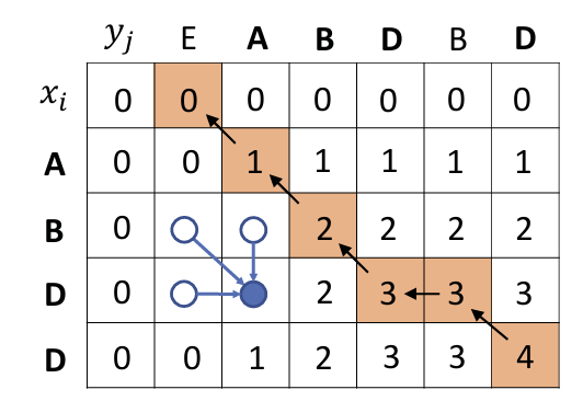
Dynamic programming [11] simplifies a problem by breaking it down to subproblems. Following the Bellman equation [37] which describes the objective function, the subproblems can be solved recursively from the initial conditions. Longest common subsequence (LCS) [31] is a classic DP algorithm that involves looking for the LCS of two known sequences $X_{m} = \{x_{0},x_{1}\ldots x_{m - 1}\}$ and $Y_{n} = \{y_{0},y_{1}\ldots y_{n - 1}\}$ . First, looking for the LCS between $X_{m}$ and $Y_{n}$ can be simplified by looking for LCSs between $X_{m}$ and $Y_{n - 1}$ , as well as $X_{m - 1}$ and $Y_{n}$ . Each of these two subproblems can be further broken down into computing the results for LCSs between $X_{m - 1}$ and $Y_{n - 1}$ . If we define $c[i,j]$ to be the length of an LCS between the sequence $X_{i}$ and $Y_{j}$ , the objective function can be represented as shown in Equation 1:

$$c[i,j] = \begin{cases} 0 & \text{if } i = 0 \text{ or } j = 0 \\ c[i-1,j-1] + 1 & \text{if } i,j > 0 \text{ and } x_{i-1} = y_{j-1} \\ \max(c[i,j-1], c[i-1,j]) & \text{if } i,j > 0 \text{ and } x_{i-1} ≠ y_{j-1} \end{cases} \tag{1}$$

Second, a DP table can be constructed based on the sequence $X_m$ and $Y_n$ to memorize the subproblem results, as shown in Figure 1. $c[i, j]$ is calculated based on its upper, left, and diagonal neighbors $c[i-1, j]$, $c[i, j-1]$, and $c[i-1, j-1]$. The first row and first column of the DP table are filled with 0. Based on this initial condition, the cells in the whole DP table can be filled out. Finally, the largest value in the table is the length of longest common subsequence and the corresponding subsequence can be found by the trace back step, as shown in the orange block chain in Figure 1.

Figure 1: DP Table for Longest Common Subsequence

2.3 DP Kernels in Genomics Pipelines

We introduce four important and time-consuming DP kernels from commonly used genomics pipelines, as shown in Figure 2. Banded Smith-Waterman (BSW) is applied in read alignment, and variants of BSW are also used for RNA and protein alignment. Pairwise Hidden Markov Model (PairHMM) is used in post-alignment variant calling. Partial Order Alignment (POA) is applied in the polishing step of assembly. Chain is used in both alignment and assembly of long read sequencing, as well as metagenomics classification. These four kernels spend $31\%$, $70\%$, $47\%$ and $75\%$ of time in corresponding sequencing pipeline stages respectively [68]. The details of these algorithms are explained as follows:

Banded Smith-Waterman (BSW) is the banded version of the Smith-Waterman [66] algorithm, which estimates the pairwise similarity between the query and reference sequences. The similarity score for a given DNA sequence is typically computed with affine-gap [52] penalties, identifying short insertions and deletions in pairwise alignments. The objective function is shown in Figure 2a, which computes three matrices H, E and F, corresponding to three edit types: match, insertion and deletion. $S$ is a similarity score between the base $X(i)$ and $Y(j)$ . $H(i,j)$ refers to the similarity score for the substring $X(0 ,i)$ and $Y(0 ,j)$ . The banded version of Smith-Waterman is applied with a maximum of $w$ insertions or deletions, illustrated as the region between black cells in Figure 2a. BSW can be computed using 8-bit or 16-bit integer arithmetic depending on the sequence length [24].

---

Match:

$$H(i,j) = \max\{H(i-1,j-1) + S(X(i),Y(j)), E(i,j), F(i,j)\}$$

Deletion: An extra base has appeared in the Read $X$, but there is no corresponding base in the reference sequence $Y$ at this position, indicating the reference sequence $Y$ is missing a base relative to the Read $X$. Penalty for the gap caused by a base absence of Y.

$$E(i+1,j) = \max\{H(i,j) - g_o, E(i,j) - g_e, 0\}$$

Insertion: An extra base has appeared in the reference sequence $Y$, but there is no corresponding base in the Read $X$ at this position, indicating that there should be an insertion occurring in Read $X$ relative to $Y$ ($X$ needs to insert a base). Penalty for a gap caused by an extra base at X.

$$F(i,j+1) = \max\{H(i,j) - g_o, F(i,j) - g_e, 0\}$$

Banded: $|i-j| \le w$

• $g_o$: gap opening penalty (open a new gap)
• $g_e$: gap extension penalty (extend the existing gap)

$S$ is a similarity score between the individual base $X(i)$ and $Y(j)$ .
$H(i,j)$ refers to the similarity score for the substring $X(0 ,i)$ and $Y(0 ,j)$.
$H(i,j)$ combines the score of the previous substring $H(i-1,j-1)$ with the current base score $S(X(i),Y(j))$ through recursion.

---

Pairwise Hidden Markov Model (PairHMM) aligns reads to candidate haplotypes identified by the De-Bruijn graph traversal. The most likely haplotype supported by the reads is identified from the pairwise alignment, which is performed by a Hidden Markov Model (HMM). The likelihood score is computed by the formula shown in Figure 2b, where $f^{M},f^{I}$ and $f^{D}$ represent match, insertion and deletion probabilities for aligning read substring $X(0 ,i)$ to haplotype substring $Y(0 ,j)$ . The weights $\alpha$ are different transition and emission parameters of the HMM. $\rho$ is the prior probability of emitting bases $X(i)$ and $Y(j)$ . The computation in PairHMM uses floating-point arithmetic [77].

---

HMM is used to calculate the likelihood probability that a sequencing read originated from a particular candidate haplotype.

$$f^M(i,j) = \rho \cdot (\alpha_{mm}f^M(i-1,j-1) + \alpha_{im}f^I(i-1,j-1) + \alpha_{dm}f^D(i-1,j-1))$$$$f^I(i,j) = \alpha_{mi}f^M(i-1,j) + \alpha_{ii}f^I(i-1,j)$$$$f^D(i,j) = \alpha_{md}f^M(i,j-1) + \alpha_{dd}f^D(i,j-1)$$

---

Partial Order Alignment (POA): In the assembly polishing step, multiple read sequences are used to construct a partial-order graph and the consensus sequence is then generated from the graph. Each unaligned sequence is aligned to the existing graph, as shown in Figure 2c. The nodes in the partial-order graph represent bases in the read sequence, and the weighted edges denote the times that the edges appear in different reads. Each cell not only depends on the upper and diagonal cells in the previous row, but also depends on earlier rows if there is an edge connecting that row with the current row in the graph. The objective function is similar to that used in BSW.

Chain: Given a set of seed pairs (anchors) shared between a pair of reads, Chain aims to group a set of collinear seed pairs into a single overlap region, as shown in Figure 2d(i). In the 1-Dimension DP table (Figure 2d(ii)), each anchor is compared with N previous anchors (default setting $N = 25$ ) to determine the best parent. However, the dependency between neighboring anchors poses difficulties for parallelism. The reordered Chain algorithm [28] compares each anchor with N subsequent anchors and updates the scores each time for them (Figure 2d(iii)).

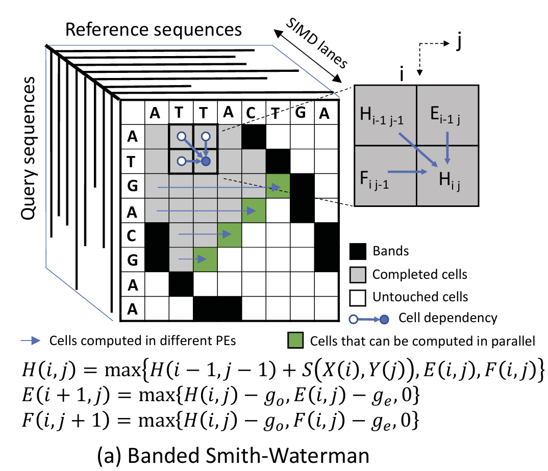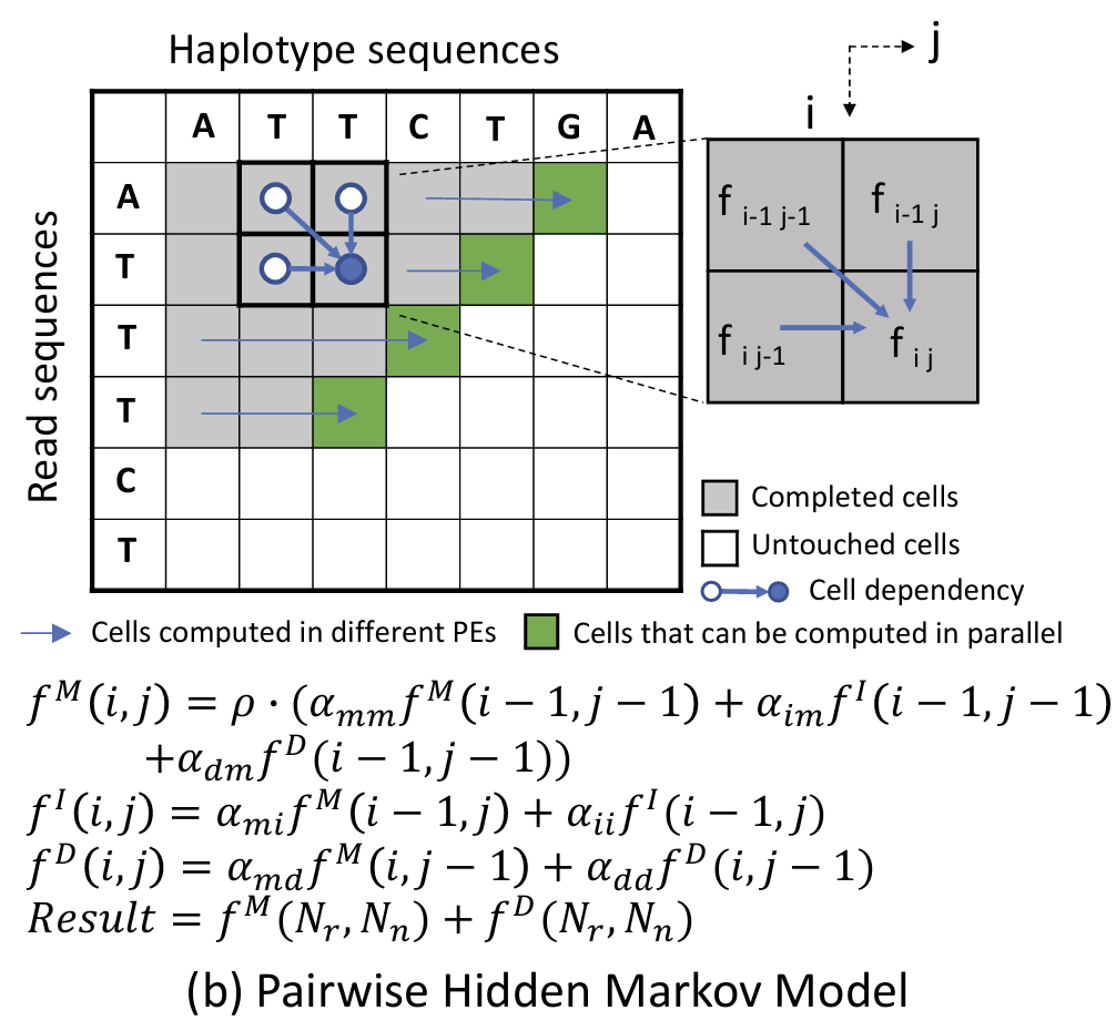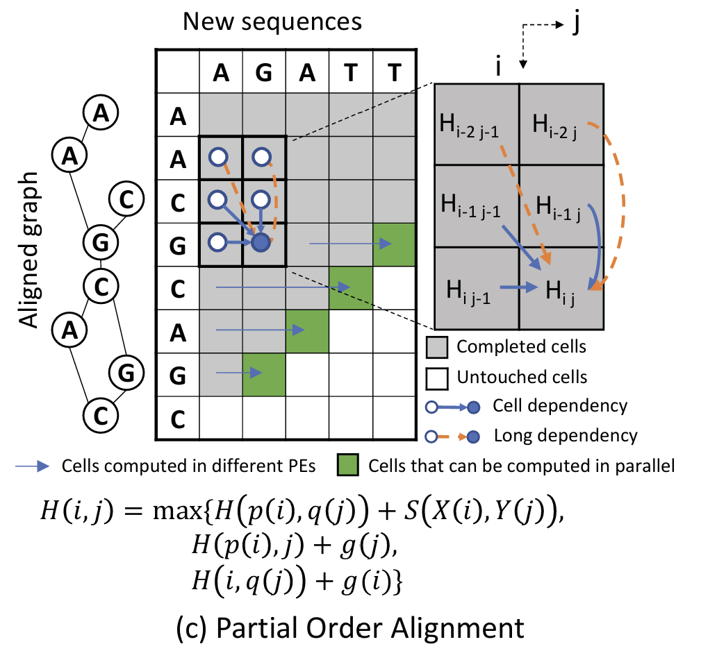
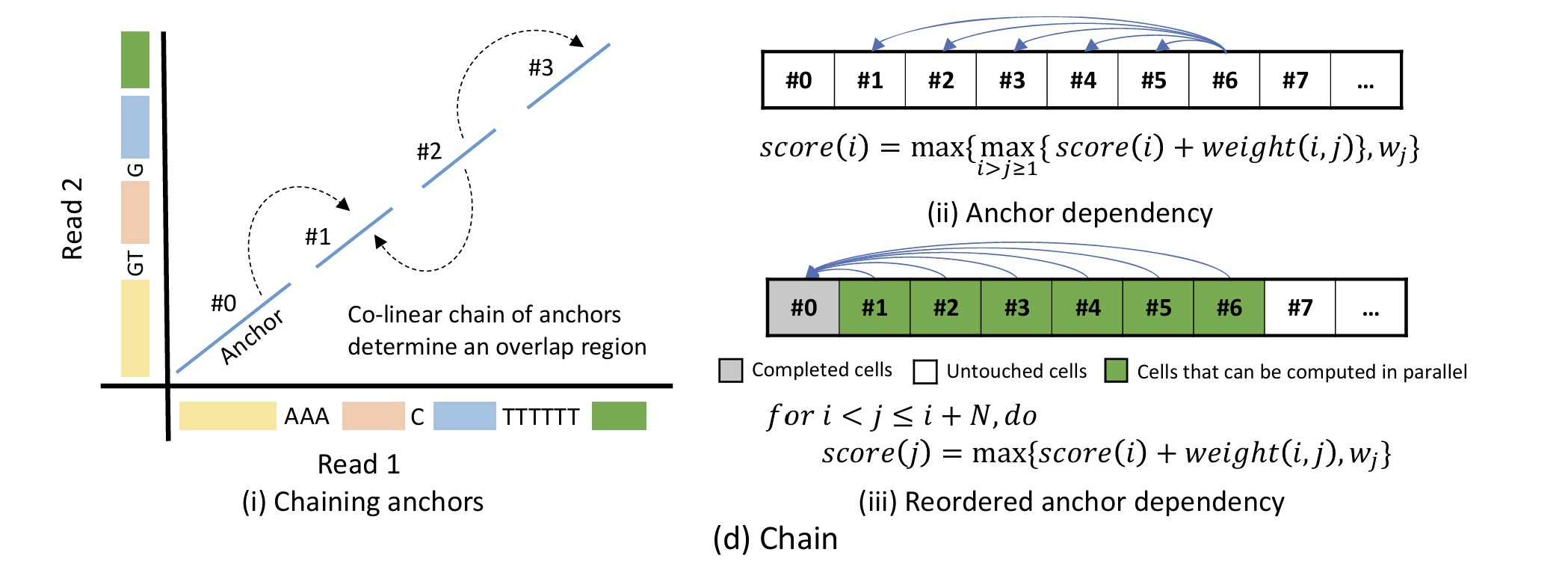
Figure 2:Black cells in BSW show the bands that limit the computing regions.Grey cells in all figures show previously computed elements and green ones on the wavefront are cells being computed in parallel. White cells show the untouched cells. Long arrows pointing to green cells show the direction that cells are being computed in different processing units in parallel. Short arrows pointing to blue circles show the dependency patterns.Cells in POA may also include long dependencies from rows other than the previous row shown by orange arrows.

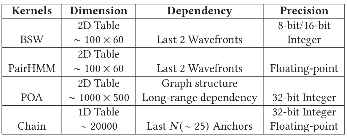
Table 1 summarizes the characteristics of four DP kernels above, including the dimension and size of DP tables, dependency patterns and arithmetic precision. BSW and PairHMM are used for short read pipelines, while POA and Chain are used in long read pipelines with larger DP tables. The first three kernels have 2-Dimension DP tables, whereas Chain has a 1-Dimension DP table. Each of these four kernels have different precision requirements, as shown in the last column.

Table 1: Characteristics of DP kernels

Figure 3: GenDP Framework

3 GENDP FRAMEWORK

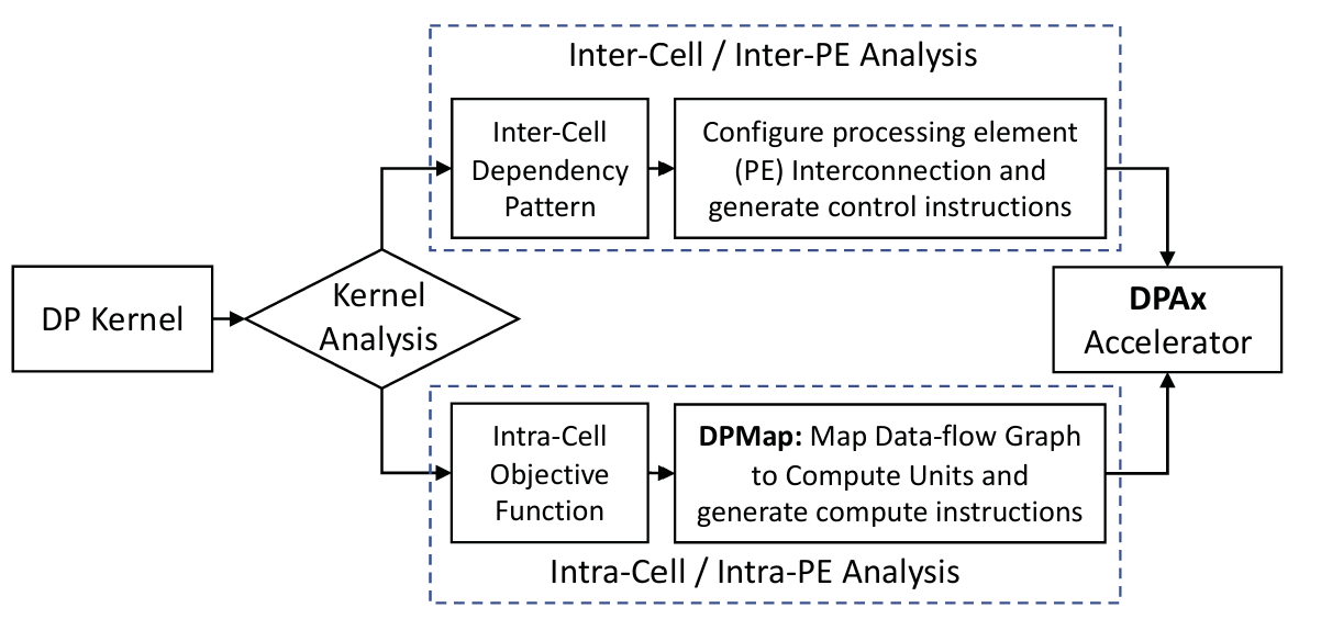
Figure 3 demonstrates the structure of the GenDP framework. For each new DP kernel, we analyze the inter-cell dependency pattern and the intra-cell objective function, as shown in the top and bottom blocks respectively in Figure 3. First, the inter-cell dependency patterns are determined by the recursion rule in the DP kernel. Based on the dependency pattern, we configure the processing element (PE) interconnection and generate the control instructions. Second, the intra-cell data-flow graph for the objective function is mapped to compute units based on the DPMap algorithm. The compute instructions are generated based on the mapping results.

Figure 4: Overview of the DPAx Architecture

3.1 Inter-Cell Dependency Pattern Supports

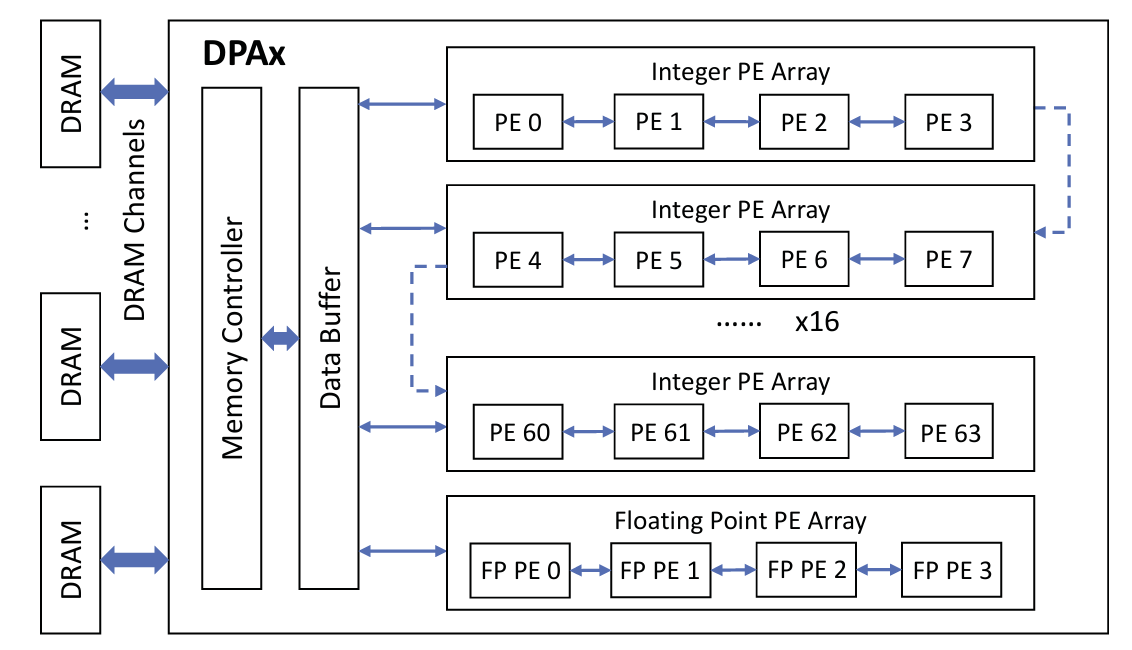
An overview of the DPAx architecture is described in Figure 4, including 16 integer PE arrays and one floating point PE array. Each PE array contains four PEs that are connected as a 1-Dimension systolic array, in which each PE can receive data from the previous PE and pass data to the next one. The interconnections of the 16 integer PE arrays are configured based on the dependency pattern of the DP kernel. The last PE in the PE array can either be connected to the first PE in the next PE array or to the data buffer directly. The 16 integer PE arrays can be concatenated and make up a large systolic array consisting of 64 PEs. Figures 5b and 5d show PE arrays of size 4 and 8 respectively.

Figure 5: Example for DP Tables and PE Interconnections

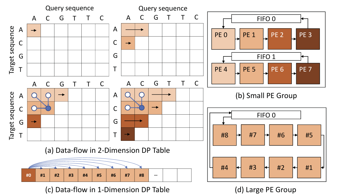
For kernels with a 2D DP Table, cells within a row are executed in the same PE. For example, rows with different colors in Figure 5 (a) are executed in PEs with corresponding colors in Figure 5 (b). Each element in the target sequence is stored in a PE statically, while elements in the query sequence are streamed through PEs in the same array. Each cell depends on results from three neighbors, the result from the left cell in the same row is stored inside the PE, while results from upper and diagonal cells in the previous row are transferred from the previous PE. First-in-First-out (FIFO) buffers connect the last and the first PEs in the array, from which the first PE (the first row in next 4-row group) acquires the dependent data from the last PE (the last row in the current 4-row group). PE array size determines how many rows can be executed in parallel.

For kernels with a 1D DP Table, cells are mapped to a large PE array as shown in Figure 5 (d). When multiple small PE arrays are connected together to form a large PE array, only the FIFO in the first PE array is utilized. For example, in the first time step, cells #1-8 in Figure 5 (c) are mapped to PEs as shown in Figure 5 (d). Cells #1-8 all depend on cell #0. Therefore, the value of cell #0 is loaded from the FIFO to each PE sequentially. During the next time step, cells #2-8 move forward to their neighboring PEs. Cell #9 is sent from the input buffer to the first PE, while cell #1 is moved out from the last PE. Meanwhile, cell #1 is loaded from the FIFO to each PE because cells #2-9 all depend on cell #1.

Long-range dependencies in the graph structure are supported by scratchpad memories (SPM) inside each PE. In a 2D DP table, usually only the result of left cell is stored in the PE. However, if a cell depends on other cells in the same row but far away, all of the candidate dependent cells need to be stored in the PE. In kernels with long-range dependencies, the result for each cell is not only stored in registers for reuse by the next cell, but also stored in SPM for potential reuse by later cells.

3.2 Intra-Cell Objective Function Mapping

In order to support DP objective functions efficiently in the PE, we design a multi-level ALU array in the compute unit. This multilevel ALU array is consistent with common compute patterns in genomics DP kernels, and reduces the register access pressure as well. The computations in the objective function are represented by data-flow graphs. DPMap partitions the data-flow graph into multiple subgraphs which can be further mapped to the ALU arrays in compute units. The partition rules, constrained by the structure of the compute unit, will be illustrated in Section 5.

4 DPAX ARCHITECTURE

4.1 Processing Element Array

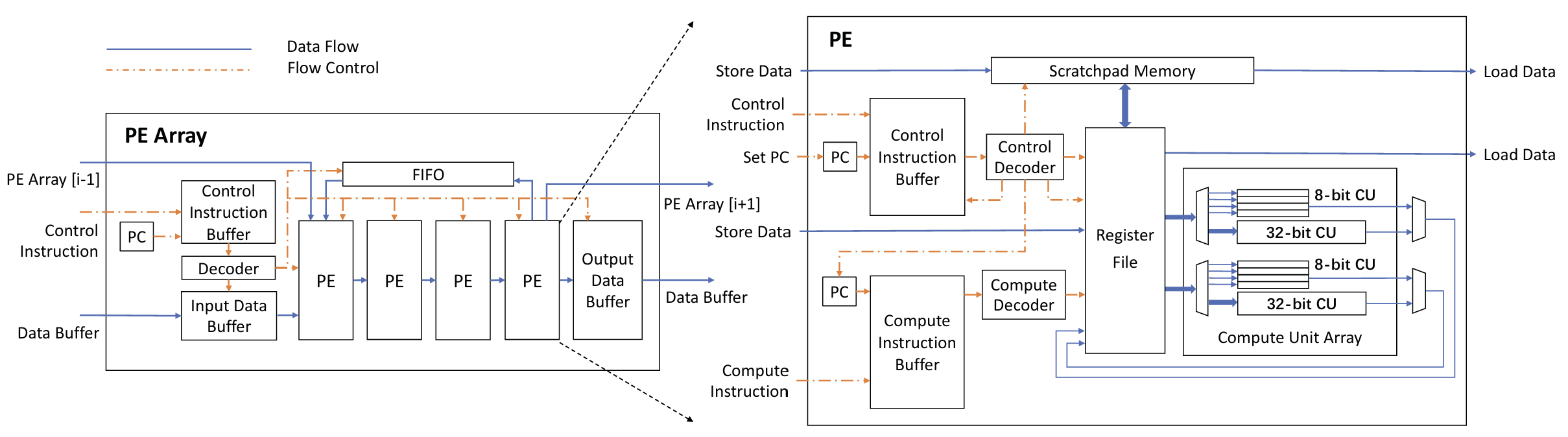
An overview of the DPAx architecture is shown in Figure 4 and discussed in the previous section. Figure 6 shows the architecture of the PE array and PE. The systolic array architecture simplifies control by allowing data-flow between neighboring PEs. However, the systolic data path alone cannot satisfy the requirements of various DP kernels. For example, POA has long-range dependencies and its dependency pattern is determined by the graph structure. The movement for such dependency requires branch instructions. Therefore, DPAx decouples the computation and control architecture to provide flexible data movements similar to decoupled access execute architectures [65]. Meanwhile, the parallelism and the massive reduction tree pattern observed in genomics DP kernels (Section 4.3) motivate the VLIW architecture.

The PE array consists of the input and output data buffers, control instruction buffer, decoder, first-in-first-out (FIFO) buffer and four PEs. PEs are connected as a systolic array and data can be passed from one PE to the next. The FIFO connects the last and first PEs. The first PE is connected to the input data buffer to receive the input sequences. The last PE stores the results to the output data buffer. The last PE in the PE array is also equipped with a dedicated port connected to the first PE in the next PE array to build a larger PE group. In Figure 6, blue solid and orange dotted lines show the data and control flow respectively.

Figure 6: PE Array Architecture

4.2 Processing Element

Each processing element (PE) is capable of running a control and a compute thread in parallel. Control and compute instructions are stored in two instruction buffers and decoded separately. Each PE contains a register file (RF) and a scratchpad memory (SPM) that store the short and long range dependencies respectively. Load and store ports are connected to the previous and next PEs. The first and last PEs are also connected to the FIFO and Input/Output Data Buffers.

Each PE is a 2-way VLIW compute unit array that can execute two independent compute instructions in parallel to exploit the instruction-level parallelism (ILP). Every PE contains two 32-bit compute units which execute the VLIW instructions. Each compute unit (CU) can either execute operations on 32-bit or four concurrent 8-bit groups of operands as a SIMD unit to make use of data-level parallelism (DLP). The SIMD unit improves the performance of low-precision kernels, e.g., BSW, where four DP tables are mapped to four SIMD lanes. The floating point PE array and PE architecture is similar to the integer one, but only supports 32-bit FP operands.

4.3 Compute Unit Design Choice

We observe that genomics DP kernels have a common reduction tree pattern as shown in Figure 7 (a) and (b). Thus, we propose a reduction tree architecture for the compute unit (CU). The outputs of the first-level ALUs are used as inputs to the next-level ALUs. The CU also contains a multiplication module for the weight calculation in the Chain kernel. Since multiplication increases the length of the CU critical path, we design it as a separate unit from the ALU reduction tree.

Figure 7: Reduction Tree Pattern in (a) BSW and (b) PairHMM Kernels. (c) (d) (e) Compute Unit Design Choices. GenDP uses the two-level reduction tree.

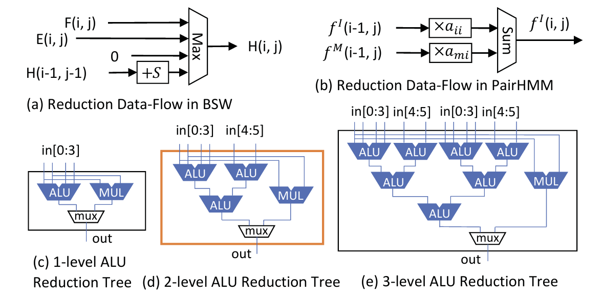
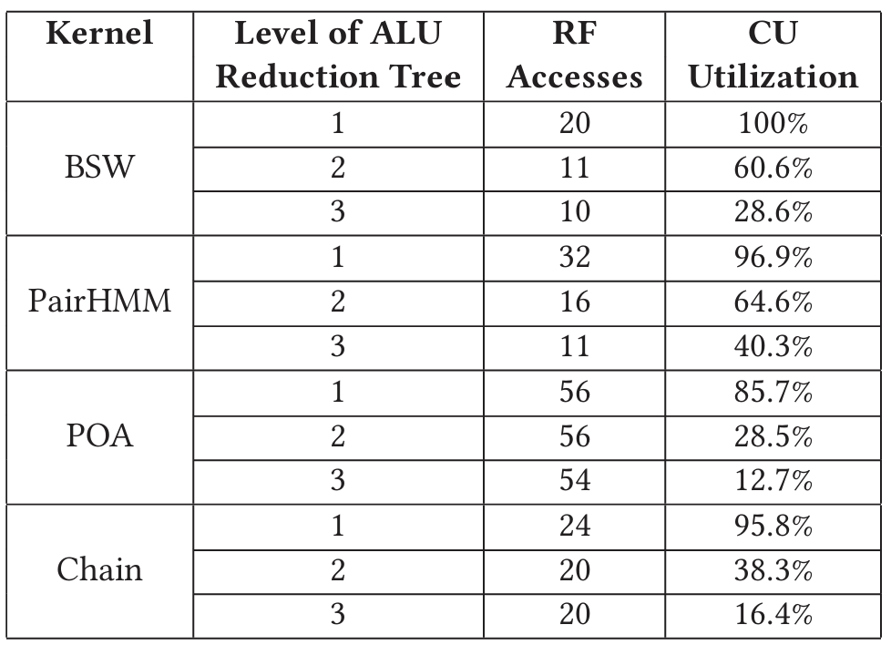
Figure 7 (c) (d) (e) shows three possible choices for the ALU reduction tree. Compared to a 1-level reduction tree, the 2-level design requires fewer register file accesses and has better balances of critical path and area; the more levels the ALU reduction tree has, the fewer times CUs need to access the register file.

Table 2 compares ALU reduction trees of 1, 2 and 3 levels, which come with 1, 3, and 7 ALUs respectively. "RF Accesses" shows the number of accesses to each RF in a single cell of the DP table. "CU Utilization" is calculated as the percentage of cycles during which each ALU is utilized in the single-cell computation. The 3-level ALU reduction tree best reduces register file accesses, but lowers the CU utilization as well. It uses more than twice as many ALUs as the 2-level tree, but hardly reduces the number of RF accesses. Thus, we pick a 2-level reduction tree for the CU design.

Table 2: ALU Reduction Trees with Different Levels

4.4 Execution Model and GenDP ISA

We adopt the following execution model for GenDP. Instructions are preloaded to the accelerator before starting a DP kernel. Each PE array runs one thread of execution, controlling the data movement between data buffers and PEs, as well as the start of the execution for each PE. Upon receiving the start flag from the PE array, each PE runs two threads of execution: control and compute. The control thread manages data movement between the SPM, register file, and the systolic data-flow between neighboring PEs. This thread also controls the start of the compute thread. The compute thread executes a compute instruction by decoding instructions, loading the data from the register file, executing computations in the CU array, and finally writing results back to the register file.

Table 3: Control Instruction Set Architecture

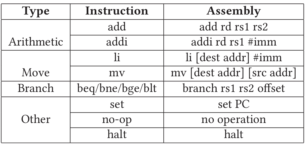
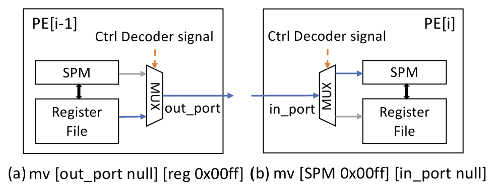
The control ISA is shown in Table 3, which is applied to the control instructions in both the PE array and PEs. Arithmetic instructions manipulate the $address$ $registers$ within the decoders. $mv$ instructions either load immediate values or move data between memory components. $branch$ instruction enables the loop iteration. $set$ instructions control the start of execution for a subsidiary component (e.g. PE arrays control PEs and PEs control CUs). Figure 8 shows an example for data movement, where two control instructions (one in each PE) are executed. PE[i-1] moves data from $0x00ff$ in the register file to its out port, while PE[i] moves data from its in $port$ to $0x00ff$ in the scratchpad memory. The delay for movements in both PEs are considered into the critical path and the movement can be done in one cycle. The control instructions are generated manually in this work.

Figure 8: Example for Data Movement

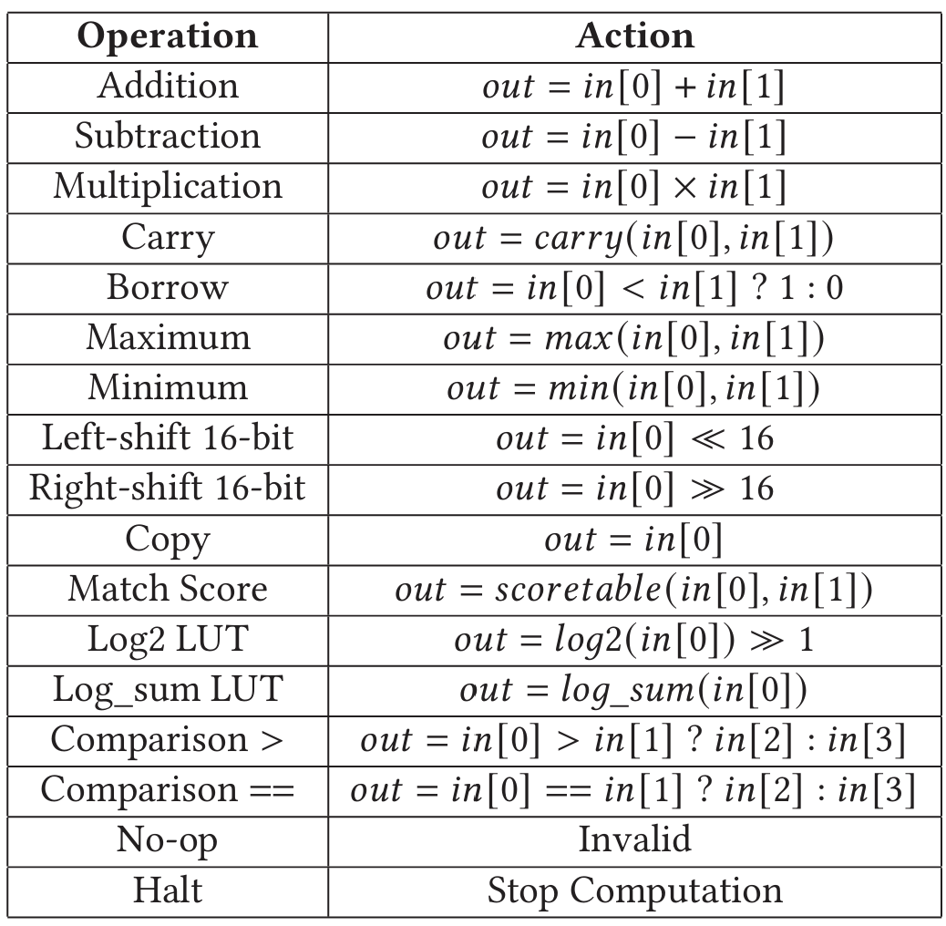
The 2-way VLIW compute instructions are executed by two compute units, each of them containing 3 operations (for 3 ALUs of the 2-level reduction tree in Figure 7 (d)) and 6 operands (4 for the top left ALU and 2 for the right one). Operations in the compute instructions are listed in Table 4. The compute instructions are generated by DPMap algorithm in Section 5.

Table 4: Compute instruction operation

5 DPMAP ALGORITHM

The DP objective function is represented as a data-flow graph (DFG). The DPMap algorithm generates compute instructions by mapping the DFG to compute units in the PE. In the DFG, a node represents an operator, while an edge shows the dependency between operators. The DFG has $|V|$ nodes $V = \{v_0...v_{|V|-1}\}$ and $|E|$ edges $E = \{e_0...e_{|E|-1}\}$. In edge $e_i = (v_m, v_n)$, the operator in node $v_n$ takes the result of $v_m$ as an operand. We define node $v_m$ as the parent of node $v_n$, and $v_n$ as the child of $v_m$. Figure 9(a) shows the DFG of the BSW kernel.

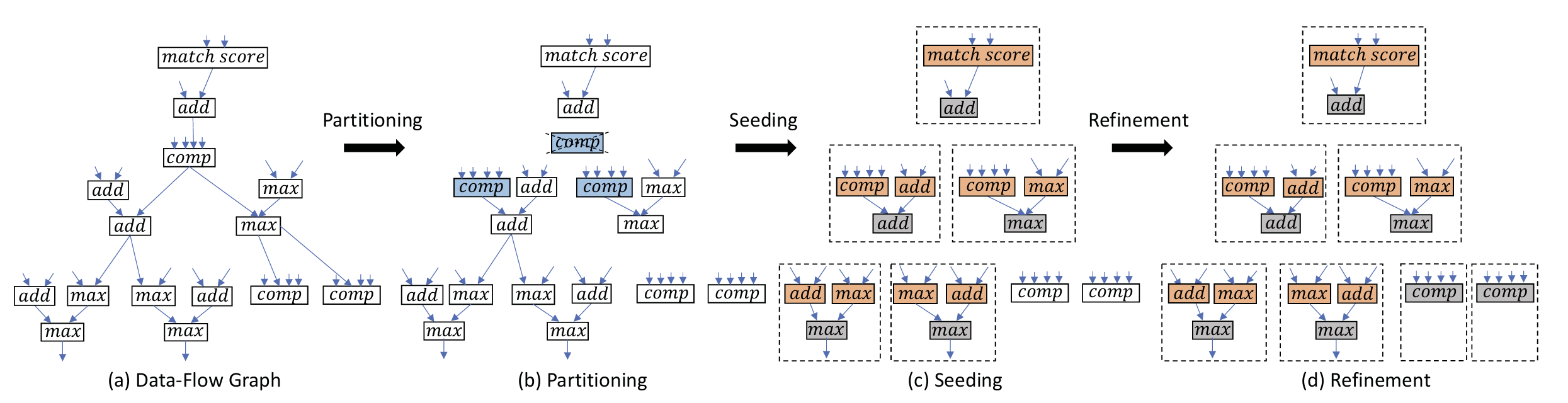Figure 9: Example for the DPMap algorithm in BSW. In (b) Partitioning, input edges of node $comp$ are removed and a $comp$ node is replicated to two $comp$ nodes, because their children both have another parent and contain commutative operations. In (c) Seeding, nodes with two parents or multiple children are located, and are grouped into subgraphs with their parents. In (d) Refinement, the remaining two $comp$ nodes are grouped into two subgraphs in the end.

BSW:

$$H(i,j) = \max\{H(i-1,j-1) + S(X(i),Y(j)), E(i,j), F(i,j)\}$$ $$E(i+1,j) = \max\{H(i,j) - g_o, E(i,j) - g_e, 0\}$$ $$F(i,j+1) = \max\{H(i,j) - g_o, F(i,j) - g_e, 0\}$$

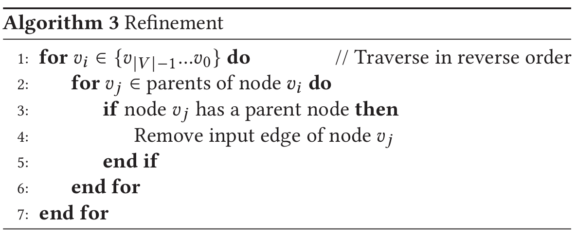
DPMap breaks the entire graph into subgraphs that contain either one multiplication or three ALU nodes (Figure 7(d)). The edges within the subgraphs represent the data movements within the compute units (CU). The edges between subgraphs represent accesses to the register file and are removed by DPMap in three steps. First, Partitioning extracts nodes that will be mapped to 4-input ALUs and multipliers, because a CU supports at most one such operation. Second, Seeding looks for nodes that could be mapped to the second level of the ALU reduction tree. Nodes with more than one parent or more than one child are selected as seeds. The seed and its parents are mapped to a CU together. After seeding, the remaining nodes have a single parent or a single child. Third, Refinement maps every two remaining nodes to the 2-level ALU tree in a CU. Figure 9 shows an example of the DPMap algorithm. Four subfigures represent the original graph and the three steps in DPMap separately. Dashed blocks represent final subgraphs.

Algorithm 1 Partitioning

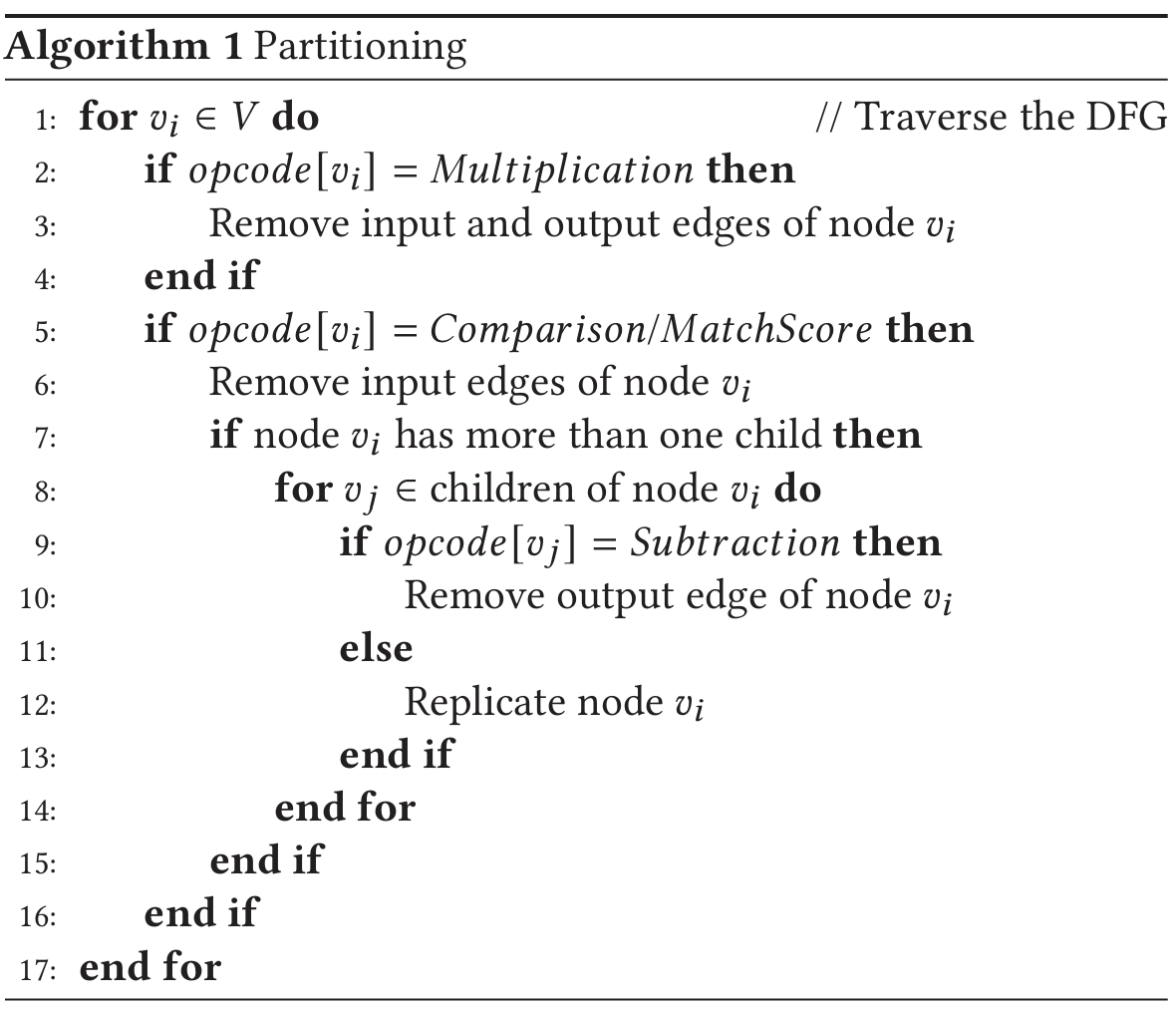
Partitioning: Algorithm 1 breaks both input and output edges connected to nodes of 4-input ALUs and Multipliers. All parent and child edges of the multiplication nodes are removed (lines 2-4). DPMap also removes the parent edges of 4-input operations (line 6). For a 4-input node that has two children, we replicate it if the operations of its children are commutative (except Subtraction) in order to decrease register file accesses (lines 8-14). After partitioning, all nodes have at most two parents.

Algorithm 2 Seeding

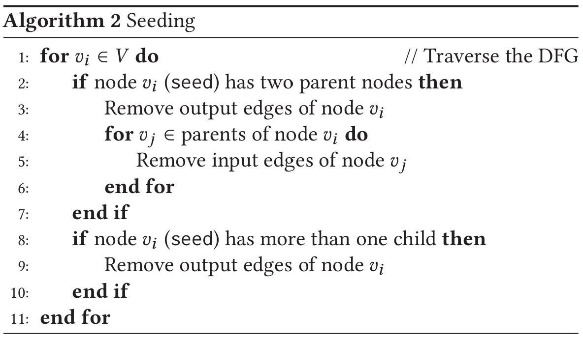
Seeding: In Algorithm 2, we look for nodes that are suitable for the second level of the ALU reduction tree and name them seeds. Nodes that have two parent nodes are located to fit the structure of the ALU reduction tree (line 2). The output edges of seeds are removed because the output of this operator will be stored to the register file (line 3). In addition, since input operands of the seed’s parents must be fetched from the register file, DPMap also removes the input edges of the seed’s parent nodes (lines 4-7). Finally, we remove the output edges of all nodes with more than one child as its outputs have to be stored in the register file (lines 9-11). At this point, all nodes have at most one parent or one child.

Refinement: Algorithm 3 traverses the DFG in reverse order. If the node has a grandparent (line 4), the edge connecting its parent and grandparent is removed to group every two nodes (line 5). In the end, all subgraphs are able to be mapped to compute units in the PE.

Algorithm 3 Refinement

6 EVALUATION METHODOLOGY

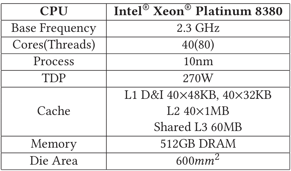
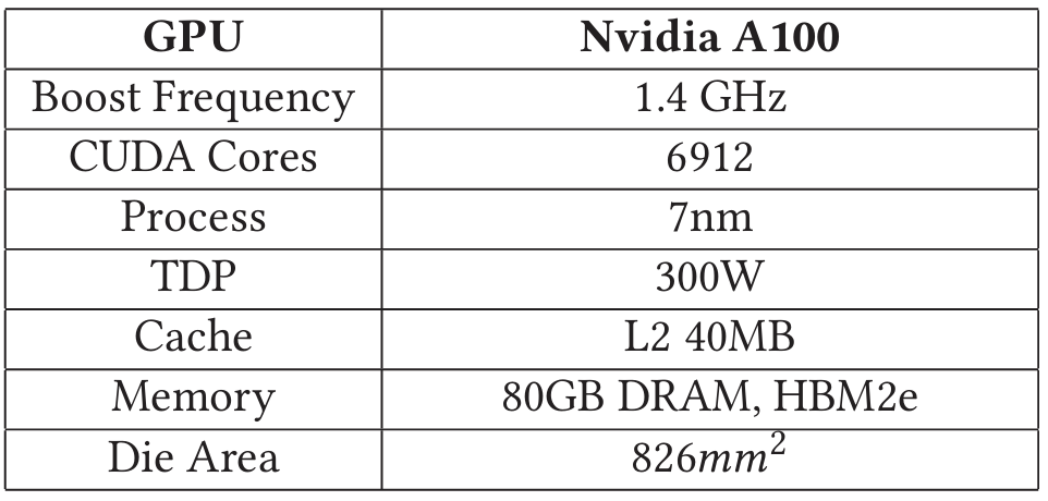
We synthesize the DPAx accelerator using the Synopsys Design Compiler in a TSMC 28nm process. We use a cycle-accurate simulator to measure the throughput of DPAx accelerator on the 4 DP kernels introduced in Section 2.3. The BSW, PairHMM and POA simulations show same results as CPU baselines. The Chain simulation implements the reordered algorithm and its accuracy is compared with CPU baseline in Table 6. We use Ramulator [36] to generate DRAM configurations and use DRAMPower [4] to measure the power by DRAM access traces. The baseline CPU and GPU configurations are shown in Table 5. All CPU baselines utilize SIMD optimizations with AVX512. The CPU die area is estimated around $600 mm^2$ [6]. We evaluate the GPU baselines on the Google Cloud Platform. The benchmark configuration for each DP kernel is detailed as follows.

Banded Smith-Waterman (BSW): BSW is evaluated on two million seed extension pairs with four 8-bit SIMD lanes on the DPAx accelerator. The dataset is obtained from the inputs to the Smith-Waterman function in BWA-MEM2 [73] using reads from the NA12878 human genome sample ERR194147, an Illumina genomics dataset consisting of short reads of 101 bp. We choose the 8-bit optimized SIMD implementation in BWA-MEM2 as the CPU baseline, and BSW implementation in GASAL2 [9] as the GPU baseline. We also compare GenDP with GenAx [24], an ASIC baseline.

Table 5: Baseline CPU and GPU Configurations

Pairwise Hidden Markov Model (PairHMM): We evaluate read-haplotype pair inputs obtained from the calcLikelihoodScore function in GATK Haplotype Caller, with BWA-MEM aligned reads for human chromosome 22 as inputs. The CPU baseline is the optimized SIMD implementation in GATK Haplotype Caller [58]. We choose the implementation in [16] as the GPU baseline. A pruning-based implementation [77] is used for both the ASIC baseline and GenDP. GenDP evaluates the scan phase in a pruning-based implementation which accounts for 97.7% of the workload. The other 2.3% of the workload is a re-computation step which is performed on the CPU. The measured performance results include time spent in re-computation on the CPU host.

Partial Order Alignment (POA): POA is evaluated by 6217 consensus tasks obtained when polishing the Flye-assembled Staphylococcus aureus genome with Minimap2-aligned ONT long reads [75]. The CPU baseline is the SIMD accelerated implementation in Racon [72] and the GPU baseline is in [5]. GenDP supports long-range dependencies of at most 128 cells away in each row of the DP table. A few ultra-long dependency (>128) cases (caused by a very long deletion in the last few input reads in a read group) account for 2.4% of the workload, and are performed on the host CPU.

Chain: We evaluate the Chain kernel using 10K reads from PacBio SMRT sequencing data of the C.elegans worm [3, 28] when computing overlaps with itself. We choose the SIMD optimized implementation in [35] as the CPU baseline and implementation in [28] as the GPU baseline. The GPU baseline and GenDP both apply the reordered Chain (Section 2.3) with N=64 in order to best utilize the parallelism and avoid large overhead of branches, thus computing $3.72\times$ more cells than the CPU baseline. We penalize the measured GPU and GenDP throughput results by $3.72\times$ to normalize them with the original CPU implementation. Our profiling results show that the reordered Chain has comparable accuracy with original Minimap2 when mapping PBSIM2 [55] simulated long reads to human genome reference T2T-CHM13 [54], as shown in Table 6.

Table 6: Chain Accuracy Comparison

7 RESULTS

7.1 DPAx Area and Power

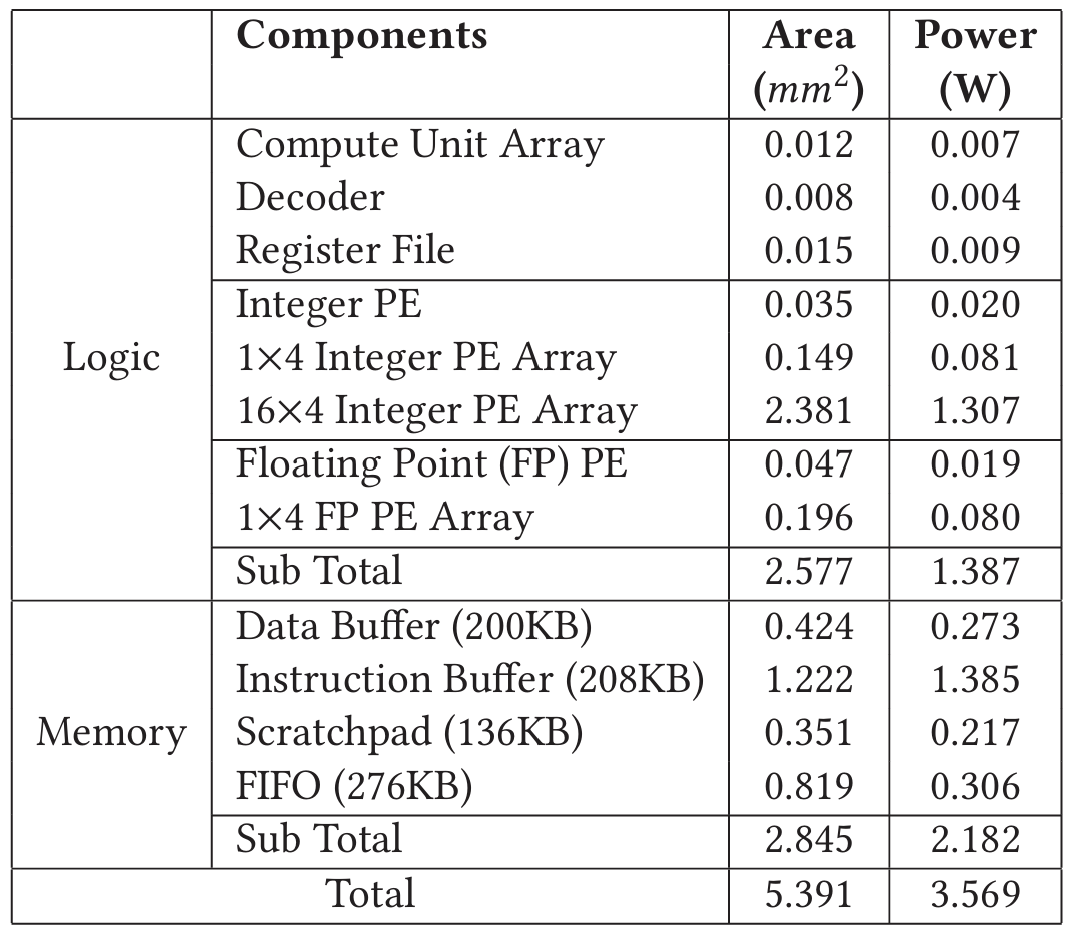
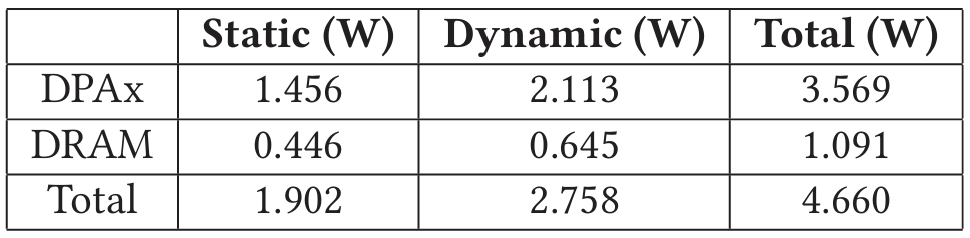
Table 7 shows the breakdown of area and power for the DPAx ASIC under a TSMC 28nm process. DPAx consumes $5.4mm^2$ in area. Within a PE, 30% of the area is taken by the register file, 22% is taken by the compute unit array, and 16% is taken by the two decoders. The other 32% of total area is consumed by SRAM, including instruction buffers and SPM. Table 8 shows the power breakdown of DPAx and DRAM in 28nm. DRAM power is averaged across the 4 kernels and DPAx power is the peak power of the ASIC.

Table 7: Breakdown of Area and Power of DPAx ASIC	Table 8: Breakdown of DPAx Power

7.2 GenDP Performance

We use throughput per unit area measured in Million Cell Updates per Second/$mm^2$ (MCUPS/$mm^2$) as a metric for performance. The area and power of CPU, GenDP and custom accelerators are scaled [67] to a 7nm process for fair comparison with GPU. GenDP is expected to run at 2GHz. Figure 10(a) shows throughput/$mm^2$ comparisons across four DP benchmarks. Overall, GenDP achieves $132.0\times$ speedup over CPU and $157.8\times$ over GPU. Figure 10(b) shows the throughput/Watt comparison between GenDP and GPU. The large speedup can be attributed to the GenDP ISA, the specialized dataflow and on-chip memory hierarchy tailored for dynamic programming.

Both the BWA-MEM2 CPU baselines and GenDP benefit from 8-bit SIMD optimizations for the BSW kernel. With AVX512, BWA-MEM2 has 64 SIMD lanes, and GenDP has 4 SIMD lanes. The PairHMM baseline applies floating point, whereas GenDP applies the pruned-based implementation using logarithm and fixed point numbers to approximate the computation and reduce complexity. The bottleneck of POA performance on GenDP is the memory accesses. First, it has the graph dependency pattern, which is more complex than other kernels. The dependency information needs to be loaded from the input data buffer to each PE. Second, downstream trace-back functions in POA need the move directions on the DP table for each cell, which requires 8-byte outputs to be written to the output data buffer from each cell. Both the input of the dependency information and the output of the move directions consume extra data movement instructions that limit POA performance on GenDP. In the Chain kernel, both performances of GPU and GenDP are penalized by $3.72\times$ for the extra cell computation.

Figure 10: GenDP Power and Performance Comparison with Baselines

7.3 Comparison with Accelerators

The GenDP framework’s goal is to build a versatile dynamic programming accelerator to support a wide range of genomics applications. Thus it sacrifices performance for programmability and supporting a broader set of kernels. A key research question is how much performance is sacrificed for generality. Figure 10(c) shows the performance of GenDP compared to available custom genomics ASIC accelerators, GenAx [24] accelerator for BSW, and pruning-based PairHMM accelerator [77]. We observe a geomean of $2.8\times$ slowdown. This can be attributed largely to area overheads, custom datapaths for cell score computation, custom data-flow, and custom precision. For example, 37.5% of the register and 40% of the SRAM are only utilized by POA but idle in other kernels, because POA is significantly more complex than the other three. A custom data-flow could specify the data bus width between neighboring PEs and propagate all the data in a single cycle, whereas GenDP needs control instructions to move data between neighboring PEs because of various data movement requirements. An accelerator for one specific kernel can implement one appropriate precision to save area. For instance, the pruning-based PairHMM ASIC utilizes 20-bit fixed-point data which satisfies the compute requirements, but GenDP has no such custom precision choice.

In addition to custom genomics ASIC accelerators, we also compare GenDP with other data-flow and spatial architectures. SoftBrain [53] is a stream data-flow accelerator, which utilizes a data-flow graph for repeated and pipelined computation, as well as stream-based commands for efficient data movements. For the 4 DP kernels discussed in Section 6, GenDP is more area-efficient and has $2.12\times$ area-normalized speedup over SoftBrain. Table 9 shows the padding overhead and SIMD utilization that limit its performance. In SoftBrain, we introduce padding to remove data hazards between pipeline stages in kernels that use 2D DP tables. SIMD utilization in DP kernels depends on both the number of SIMD lanes as well as the length of input sequences. In addition, kernels with a graph structure like POA gain little from the SIMD parallelism because the number of edges connected to each node varies in the graph. Intra-cell pipelining is not well suited for POA because the intra-cell iterative blocks are sequentially computed and dependent on each other, leading to intra-cell pipeline hazards. Inter-cell pipelining also provides limited benefits because there is a variable number of block iterations within each cell (determined by the number of edges connected to the current node).

Table 9: Benchmark implementation on SoftBrain

	Dimen-sion	Pipe. Stages	Padding Overhead	SIMD Lanes(Util.)	GenDP Speedup
BSW	2D	3	9.9%	8(42.2%)	2.24x
PairHMM	2D	4	15.7%	2(95.9%)	1.13x
POA	Graph	1	0	1(100%)	10.74x
Chain	1D	10	0	2(73%)	0.75x

Triggered instruction architecture (TIA) [56] eliminates the program counter and branch instructions by predication, and exploits the locality in the spatial algorithms by using a PE array with mesh topology. However, the area and timing complexity of the trigger scheduler imposes a restriction on the number of triggered instructions (TI). For example, an implementation of edit distance scoring-based DP on top of TIA requires two PEs for 11 TIs [69]. A similar mapping strategy used on the DP kernels in Section 6 requires multiple PEs to compute the objective function in a single DP cell, limiting the benefits obtained from a spatial architecture like TIA. The number of TIs and PEs required by objective functions in each DP kernel is listed in Table 10.

Table 10: Triggered Instruction (TI) Required on TIA

Kernel	BSW	PairHMM	POA	Chain
Number of TIs required	30	45	90	47
Number of PEs required	5	8	16	8

In summary, GenDP balances well the specialization and generality trade-off for dynamic programming acceleration. Custom ASIC accelerators achieve better performance but are less programmable. SoftBrain, with reconfigurable networks, cannot efficiently support the DP kernels described in this work because of parallelism overhead and pipeline hazards. TIA reduces control instructions and exploits the spatial locality but is not well suited for compute-intensive DP kernels with complex scoring schemes.

7.4 ISA Analysis

GenDP has a more efficient ISA for DP algorithms than general-purpose processors. We compare the number of compute instructions required per cell update in GenDP ISA to riscv64 and x86-64 ISA. The riscv64 and x86-64 instruction counts are obtained using riscv64-unknown-elf-g++ and g++ compilers respectively. Among four kernels, the instruction counts on GenDP are reduced by $8.1\times$ and $4.0\times$ on average when compared with riscv64 and x86-64, shown in Figure 10(d). The efficiency of GenDP instructions is affected by compute unit utilization, as shown in Table 2.

Several advantages of GenDP ISA are shown as follows: First, GenDP applies the VLIW architecture, where one instruction contains opcodes for 6 ALUs in the compute unit (CU) array. The ALU reduction tree in the CU fits the compute characteristics of DP kernels well. GenDP has an average 48% VLIW utilization among 4 kernels, shown in Table 11. The multiplication and conditional operations in Chain and POA could only be mapped to 4-input ALUs in DPAx, which limits the VLIW utilization. Meanwhile, During the execution in POA, 14.3% of the CUs are idle because of the complex dependency pattern of POA. Second, GenDP's ISA includes several custom operations such as Comparison, Max/Min and Lookup Table (LUT). In Chain, GenDP uses a special instruction for the LUT. In comparison, riscv64 and x86-64 need 14 and 7 instructions respectively for this LUT implementation. Third, the systolic array architecture provides spatial locality and saves many register-to-register operations. Meanwhile, DPAx has a memory hierarchy design with FIFO and scratchpad memory, which cache intermediate values for inter-cell communication and reduce the memory access to DRAM.

Table 11: VLIW Utilization

Kernel	BSW	PairHMM	Chain	POA
Utilization	60.6%	64.6%	38.3%	28.5%

7.5 Scalability

With 8-channel DDR4-2400 DRAM (153.2 GB/s peak bandwidth), GenDP could scale up to 64 DPAx tiles and achieve $6.17\times$ raw performance speedup over the GPU baseline, shown in Table 12. The area of GenDP is scaled [67] to 7nm to make a fair comparison with the GPU baseline.

7.6 Generality and Limitation

In addition to these four DP kernels within the commonly used sequencing pipelines, the GenDP framework also supports other DP algorithms in either genomics or broader fields. This section discusses the generality and limitation of GenDP.

Table 12: GenDP and GPU Raw Performance Comparison

	Area($mm^2$)	Raw Perf.(GCUPS)	Speedup
NVIDIA A100 GPU	826.0	48.3	1
GenDP (64 tiles)	44.3	297.5	6.17x

7.6.1 Dependency range. DP algorithms could be categorized into near-range (e.g., neighboring dependency pattern), limited long-range (e.g., dependency distance within 128) and ultra long-range (e.g., dependency distance longer than 128). GenDP could efficiently support near-range and long-range dependencies by fine-grained spatial locality design, such as the systolic array and scratchpad memory in the PE. GenDP also supports ultra long-range dependencies but needs to access these data through DRAM because the on-chip buffer is not large enough. However, the ultra long-range dependencies are usually rare, for example, POA only has 2.4% workload with dependency distances longer than 128, which are performed on the host CPU in simulation.

7.6.2 Active region. GenDP requires to specify the active regions in the DP table before the computation starts. For example, GenDP supports the static band choice in the DP table but does not support adaptive or dynamic band choice. In these cases, GenDP could choose a larger tiled static region that covers the adaptive bands but will sacrifice some performance.

7.6.3 Objective function. GenDP ISA supports most computations in the commonly used genomics pipeline, including local, global and semi-global approximate string matching as well as linear, affine, and convex scoring modes mentioned in Section 1. It also supports DP algorithms in other fields such as speech detection and robot motion planning.

7.6.4 Multi-precision arithmetic. DP kernels utilize computations of different precisions. For example, BSW can be computed using 8-bit or 16-bit precision depending on the sequence length. Computations in POA and Chain are in 32-bit integer format and PairHMM requires both integer and floating-point computation. DPAx has both integer and floating-point PEs. The integer PEs support 32-bit and 8-bit integer arithmetic, and also support 64-bit and 16-bit basic operations such as addition, subtraction, and multiplication by using two parallel compute units.

[Figure 11 Placeholder: GenDP Instruction and Performance on DTW and BF benchmarks]

Figure 11: GenDP Instruction and Performance on DTW and BF benchmarks

7.6.5 Broader field. Dynamic Time Warping (DTW) measures the similarity between two temporal sequences, which could be utilized for nanopore signal basecalling [23] and speech detection [12]. DTW has near-range dependency pattern similar to Smith-Waterman. Bellman-Ford (BF), a shortest path search algorithm, is commonly used for robotic motion planning applications. BF has a graph-based dependency pattern where the long-range dependencies within a certain distance could be efficiently supported by GenDP and the ultra-long range dependencies need accesses through DRAM. GenDP supports both objective functions of DTW and BF. Their performance and instruction comparisons with GPU [1, 64] are shown in Figure 11.

8 RELATED WORK

Dynamic Programming Accelerators in Genomics: Many custom genomics accelerators have been proposed to boost the performance of DP kernels in genomics pipelines, which significantly improve the performance over commodity hardware. However, these accelerators only support a single genomics kernel and must be customized and combined to support different stages of genomics pipelines. This increases both design cost and complexity. For example, [18-20, 24, 25, 45, 47, 70] are customized for read alignment and SquiggleFilter [23] is optimized for basecalling. GenASM [14] converts the DP objective function into bit-wise operations such as AND, OR, and SHIFT. Although GenASM partially supports the affine gap penalty model [52], bit-wise operations inherently fail to implement all the complex objective functions needed in different stages of genomics pipelines. SeGraM [15] extends GenASM to sequence-to-graph mapping and supports seeding, but supports limited DP objective functions as well. Race Logic [47] utilizes the race conditions in the circuit to accelerate the edit distance function in the bioinformatics field such as DNA sequence alignment and protein string comparison. However, other DP kernels such as PairHMM and Chain are not edit distance problems and have more complicated objective functions and higher numeric precision requirements. It is challenging to map such kernels to the Race Logic accelerator. GenDP aims to fill this gap and proposes a generalized acceleration framework that can be applied to accelerate the various flavors of dynamic programming common in genomics pipelines.

Besides genomics applications, dynamic programming algorithms are also accelerated in other domains, such as shortest path in robot motion planning [51]. There has also been industry interest in DP acceleration. For example, NVIDIA recently announced the dynamic programming instructions (DPX) in the Hopper architecture [8], but the corresponding products and CUDA library have not been released yet.

Domain Specific Accelerators in Genomics: Several domain specific accelerators have been explored for databases [76], machine learning [21, 33] and graph processing [22, 30]. However, there has been little work on domain specific accelerators for genomics. Based on the insight that data manipulation operations are also common in genomics pipelines, Genesis [29] proposes a domain-specific acceleration framework customized for data manipulation operations in genome sequencing analysis. Genesis uses an extended SQL as a domain specific language and provides the relevant hardware libraries. The framework is evaluated on AWS cloud FPGA and achieves up to $19.3\times$ speedup over the 16-thread CPU baseline. However, the hardware modules only cover database operations for data manipulation and users need to add custom modules for different genomics pipelines. In contrast, different from Genesis’s target, GenDP focuses on dynamic programming acceleration in genomics pipelines.

General Accelerators: There are also several works that have identified common compute and memory access patterns across both regular and irregular workloads and proposed reconfigurable, spacial and dataflow architectures for these patterns [27, 53, 56, 59]. But these accelerators are mostly optimized for data-parallel or data-intensive applications and not suitable for dynamic programming kernels. Plasticine [59] is a spatially reconfigurable architecture for parallel patterns, which supports broad applications, but has lower functional unit utilization on data-dependent applications such as PageRank (3.9%) and BFS (3.1%) than data-parallel applications (~50%). SoftBrain [53] and TIA [56] are discussed in Section 7.3.

9 CONCLUSION

In order to support general-purpose acceleration for genomics kernels in the commonly used sequencing pipelines, this work presented GenDP, a programmable dynamic programming acceleration framework, including DPAx, a systolic array-based DP accelerator, and DPMap, a graph partitioning algorithm to map DP kernels to the accelerator. DPAx supports multiple dependency patterns through flexible PE interconnections and different DP objective functions using programmable compute units. GenDP is evaluated on four important genomics kernels, achieving $157.8\times$ throughput/$mm^2$ and $5.1\times$ throughput/Watt compared to GPU, and $132.0\times$ throughput/$mm^2$ over CPU baselines, and is also extended to DP algorithms in broader fields.

ACKNOWLEDGMENTS

We thank the anonymous reviewers for their suggestions which helped improve this paper. This work was supported in part by the NSF under the CAREER-1652294 and NSF-1908601 awards, and the Applications Driving Architectures (ADA) Research Center, a JUMP Center co-sponsored by SRC and DARPA.

A ARTIFACT APPENDIX

A.1 Abstract

This document briefly describes how to reproduce the main performance results of this paper in Figure 10 (a) and (c). The instructions in this document include 1) how to download the datasets, 2) how to run CPU/GPU baselines, 3) how to run GenDP simulations. The source code and instructions are accessible from GitHub. The expected results are shown in Table 13, 14 and 15.

A.2 Artifact check-list (meta-information)

• Algorithm: Banded Smith-Waterman (BSW), Chain, Pairwise Hidden Markov Model (PairHMM), Partial Order Alignment (POA).
• Program: C++ and Python
• Compilation: g++ 8.3.1 and Intel® oneAPI DPC++/C++ Compiler 2021.8.0
• Data sets: Illumina NA12878 human genome sample ERR194147 (BSW), PacBio SMRT sequencing data of the C.elegans worm (Chain), human chromosome 22 (PairHMM), Flye-assembled Staphylococcus aureus genome (POA).
• Hardware: Intel CPU with >= 16G memory and >= 40G storage, and NVIDIA GPU.
• Execution: Bash script for compilation and execution
• Metrics: Throughput: cell updates per second
• Output: CPU/GPU runtime and GenDP throughput
• Experiments: CPU/GPU baselines and GenDP simulation for 4 benchmarks (BSW, Chain, PairHMM and POA)
• How much disk space required (approximately)?: 40G
• How much time is needed to prepare workflow (approximately)?: ~ 1 hour
• How much time is needed to complete experiments (approximately)?: ~ 24 hours
• Publicly available?: Yes.
• Archived (provide DOI)?: https://doi.org/10.5281/zenodo.7792246

A.3 Description

A.3.1 How to access. The artifact could be accessed from GitHub and Zenodo.

A.3.2 Hardware dependencies.

(1) Intel CPU and NVIDIA GPU (2) 16G memory and 40G storage

A.3.3 Software dependencies.

(1) Linux OS (2) gcc >= 8.3.1 (3) cmake >= 3.16.0 (4) OpenMP >= 201511 (5) Intel® DPC++/C++ Compiler >= 2021.8.0 (6) ZLIB >= 1.2.8 (7) CUDA >= 10.0 (8) Python >= 3.7.9 (9) numactl >= 2.0.0

A.3.4 Data sets. The list below shows the details of datasets and the table shows the approximate simulation time and corresponding input size. BSW simulation is fast and the default setting is entire dataset.

• BSW: Illumina NA12878 human genome sample ERR194147 (1932254 short reads with length $<= 128$)
• Chain: PacBio SMRT sequencing data of the C.elegans worm (10000 long reads)
• PairHMM: Human chromosome 22 (1420266 short reads)
• POA: Flye-assembled Staphylococcus aureus genome (6216 consensuses, each including 10 ~ 100 long reads)

A.4 Installation

Download the code base from GitHub and install Intel DPC++/C++ Compiler (ICX).

A.5 Experiment workflow

Please follow the instructions on GitHub.

Step 1: Check System Requirements Step 2: Download Repository and Data sets (~ 10 min) Step 3: Run CPU Baselines (~ 10 min) Step 4: Run GPU Baselines (~ 10 min) Step 5: Run GenDP Simulation (~ 24 hours)

Table 16 shows the relationship between data sets size and simulation time. We recommend to run scripts for ~ 6 hours or ~ 24 hours.