6 Locus

Locus: A Variation-Aware Accelerator for Sequence-to-Graph Mapping on Pangenome Graphs

PDF

superbubble detect algorithm

Abstract

Pangenome graphs are emerging as an alternative to single linear references for population-scale genomic analysis because they can explicitly encode population diversity and genetic variation. This richer representation helps reduce reference bias and improve read mapping and variant analysis. However, leveraging these benefits requires moving beyond traditional sequence-to-sequence mapping to sequence-to-graph mapping, which substantially increases computational complexity. This complexity introduces two key challenges. First, additional processing stages, such as linear chaining and graph chaining, are needed to capture genetic variation in pangenome graphs, causing intermediate data movement to dominate off-chip memory access. Second, genetic variations encoded as bubbles in pangenome graphs further increase irregularity and hinder parallelization.

In this paper, we propose Locus, an efficient accelerator for sequence-to-graph mapping on pangenome graphs. The key idea behind Locus is to address the increased intermediate data movement and computational irregularity introduced by genetic variation in pangenome graphs. Specifically, we develop a bubble-aware partitioning algorithm that groups variation bubbles while preserving workload balance. In addition, we propose a variation-aware dataflow and a flexible accelerator architecture that jointly fuse multiple sequence-to-graph mapping stages, thereby reducing intermediate data movement and off-chip memory access. We simulated our design using GRCh38 pangenome datasets [1]. Simulation results show that Locus achieves $2.1 \times$ the throughput and $1.2 \times$ the energy efficiency over the state-of-the-art accelerators [2]–[8], reduces DRAM traffic by $96\%$, and produces near-identical results to software Minigraph.

I. INTRODUCTION

Pangenome graphs have emerged as an alternative to single linear references for population-scale genomic analysis [9]–[11], as they can explicitly encode population diversity and genetic variation. This richer representation reduces the reference bias inherent in linear mapping and enables more accurate variant calling across diverse populations [12], [13]. However, adopting pangenome graphs shifts genomic analysis from traditional sequence-to-sequence mapping (S2S) [6], [14], [15] to sequence-to-graph mapping (S2G), which aligns sequencing reads to a graph-based genome reference by identifying candidate matches and tracing paths through variant branches to determine each read’s most likely genomic origin [16].

The fundamental distinction between a pangenome graph and a linear reference is the representation of genetic variation. In a pangenome graph, variation is encoded as bubbles, where the graph branches into multiple alternative paths that capture different alleles or haplotypes. To map reads across these alternative paths, sequence-to-graph mapping uses linear chaining and graph chaining to connect candidate matches while handling graph-structured variation. Based on our profiling of the HPRC pangenome graph [9] across all 22 human autosomes, approximately $40\%$ of graph nodes reside in bubble regions. Compared with non-bubble regions, bubbles contain longer sequences on average and exhibit higher vertex degree, since each bubble contains multiple alternative paths. These properties introduce two key computational challenges.

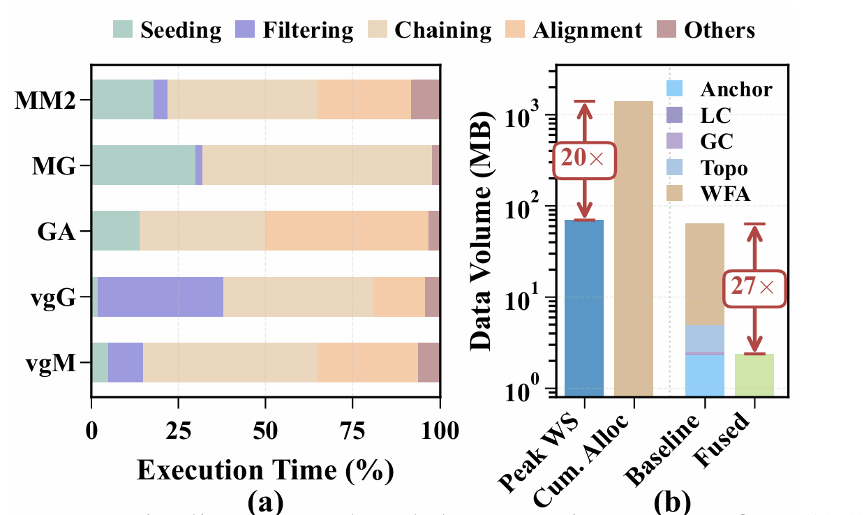
Fig. 1: (a) Pipeline stage breakdown varies across five S2G mappers, and (b) DRAM traffic comparison.

First, unlike S2S mapping, S2G mapping introduces additional stages, leading to substantially higher DRAM traffic for intermediate data. Specifically, seeding produces anchors, which are consumed by linear chaining to construct candidate chains, and these chains are subsequently used by graph chaining to extend mapping across graph paths. This stage-by-stage dependence requires repeated movement of intermediate results, making intermediate data transfer a dominant component of memory traffic. As Figure 1(a) shows, no single stage dominates across S2G mappers, and our analysis shows that intermediate data exchanged between S2G stages accounts for $86\%$ of total DRAM access (Figure 1(b)). Prior acceleration efforts have primarily targeted an individual S2S or S2G stage. For instance, GenDP [4] introduces reconfigurable compute units and a partitioning scheme to support diverse dynamic programming (DP) kernels for alignment and chaining. TALCO [7] develops a tiling strategy to improve the efficiency of DP score computation and storage during alignment. Harp [5] leverages the quasi-sequential structure of genome graphs and employs a compact on-chip data structure to accelerate chaining and filtering. SeGraM [2] presents the first minimizer-based seeding accelerator integrated with bitvector-based alignment. In general, alignment accelerators focus on wavefront-based algorithms with dense DP computation [17], whereas chaining-stage optimizations target the sparse dependency structure among anchors [16].

Moreover, compared with conventional graphs, pangenome graphs introduce additional challenges for workload balancing. In pangenome graphs, each node may carry a sequence of variable length, leading to nonuniform computational cost across nodes. In addition, pangenome graphs contain bubble regions that explicitly represent genetic variation, whereas traditional graphs more commonly exhibit power-law structural properties. Although substantial prior work [18]–[21] has studied graph partitioning, most existing approaches focus primarily on minimizing edge cuts or vertex cuts. Such objectives are not sufficient for pangenome graphs: blindly minimizing cuts can split bubble regions across partitions, increasing inter-partition communication and breaking the strong dependencies among alternative paths within a bubble. To preserve locality and efficiently process variation-rich regions, pangenome graphs require a new bubble-aware partitioning algorithm.

In this paper, we propose Locus, an efficient accelerator architecture for sequence-to-graph mapping on pangenome graphs. Our key observation is that, while pangenome graphs provide a powerful way to represent genetic variation, they also introduce additional processing stages and irregular branch connectivity across nodes. These characteristics increase intermediate data movement between stages and complicate efficient parallel execution. To address these challenges, Locus combines new algorithms and dataflows to fuse multiple computational stages by retaining intermediate data on chip, together with a new graph partitioning algorithm that improves parallelism and workload balance.

• We develop an analytical model to characterize the complex memory-access behavior of sequence-to-graph mapping. Building on this model, we propose a new graph partitioning algorithm that detects bubble regions in pangenome graphs and preserves their locality. This design keeps long-range dependencies within each partition while maintaining workload balance across partitions.
• We propose a unified accelerator architecture that supports the diverse computation and communication patterns across different stages of sequence-to-graph mapping. This design creates opportunities to retain intermediate data on chip, enabling fine-grained pipelined execution across stages. In addition, we develop a new dataflow that maximizes both temporal and spatial data reuse for sequence-to-graph mapping.
• We evaluate Locus using HPRC pangenome datasets [9]. The results show that Locus achieves $2.1\times$ the throughput and $1.2\times$ the energy efficiency, and lowers DRAM traffic by $96\%$ compared with state-of-the-art accelerators, while producing near-identical results to software Minigraph.

II. BACKGROUND AND MOTIVATION

A. Pangenome Graph

The concept of representing genetic variation [22], [23] as a graph rather than as a linear sequence has evolved significantly over the past decade. Early work on variation graphs [24] (i.e., pangenome graphs, as shown in Figure 2) demonstrated that encoding known variants within the reference structure can improve read mapping accuracy, particularly for populations underrepresented in the original reference assembly. The development of the Graphical Fragment Assembly (GFA) format [25], [26] further standardized this representation: each segment (i.e., node) stores a DNA subsequence, each directed edge connects segments, and each named path traces a complete chromosome sequence. This format has been adopted by major pangenome construction pipelines, including Minigraph-Cactus [27], PGBG [28], and the Human Pangenome Reference Consortium (HPRC) [9].

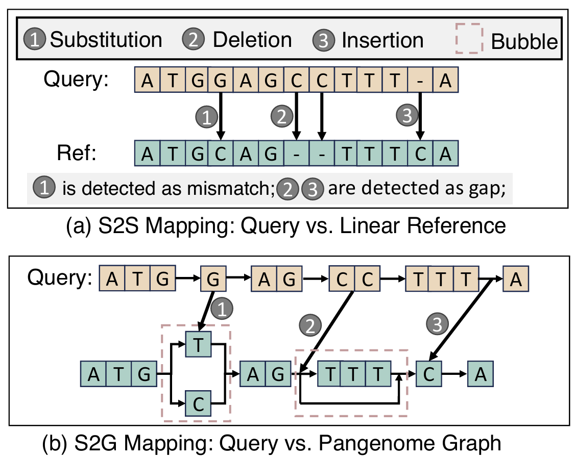
Fig. 2: (a) Sequence-to-sequence mapping and (b) sequence-to-graph mapping.

In this work, we profile the HPRC GRCh38 pangenome graph as a case study, which incorporates 94 diverse chromosome haplotypes spanning 3.1 billion base pairs. Unlike conventional graphs in social networks or recommendation systems [29], [30], which often exhibit power-law degree distributions with a small number of highly connected nodes, pangenome graphs inherit the near-linear topology of chromosomal DNA. Specifically, they consist of a dominant backbone linear chain with localized branching at sites of genetic variation, forming bubble structures. This distinctive topology introduces new challenges for S2G mapping.

Linear and bubble regions. Given the structural characteristics of pangenome graphs, nodes can be naturally categorized into two types [10], [11]. A bubble node is a node that lies inside a superbubble, that is, a subgraph that diverges from a single entry vertex into alternative paths and reconverges at a single exit vertex [31]. All remaining nodes are sequential and lie on the unique backbone path conserved across chromosomes. Branch and merge vertices bound each bubble, while the alternative alleles inside it count as bubble nodes even though their individual in- and out-degrees are one. This structural dichotomy was introduced in the context of assembly graphs [?] and later extended to variation graphs. Using the PGBG toolkit [28], we profiled the full human pangenome graph across all 22 autosomes and found a remarkably stable proportion of bubble regions: Sequential nodes comprise $59.7\% \pm 1.5\%$ of all nodes across chromosomes, with an average node length of $\sim 50\mathrm{bp}$ whereas bubble nodes comprise $40.3\% \pm 1.5\%$ with an average node length of $\sim 108\mathrm{bp}$.

Although bubble regions account for only about $40\%$ of nodes, they contain approximately $60\%$ of the total sequence bases because bubble nodes encode full alternative allele sequences and are, on average, roughly twice as long as sequential nodes in our profiling. This $60/40$ distribution is not unique to a single chromosome; it remains consistent within $\pm 2\%$ across all autosomes from chr1 to chr22, reflecting the underlying distribution of human genetic variation observed in large-scale sequencing studies [23].

B. Sequence-to-Graph Mapping Pipeline

Mapping query sequences to pangenome graphs has been addressed by diverse algorithmic strategies over the past decade. Early methods such as BwBBLE [32] extended FMindex techniques to graph structures, enabling exact matching but struggling with the combinatorial explosion of paths in bubble regions. More recent tools have converged on a multi-stage pipeline architecture that balances sensitivity and computational tractability. GraphAligner [33] proposed bitvector alignment for long reads on graphs. The vg toolkit [12] introduced the GBWT index [34] for efficient haplotypeaware queries, with vg Giraffe [35] optimizing for short-read throughput. Minigraph [26] targets long reads and assembly sequences with a chaining-first approach that minimizes expensive alignment operations. Despite their algorithmic differences, these tools share a common five-stage pipeline structure and face a common bottleneck: bubble regions impose disproportionate computational and memory costs at every stage, from chain fragmentation in LC to repeated subgraph traversal in GC and enlarged wavefront buffers in alignment. We describe this pipeline following the Minigraph implementation that serves as our algorithmic baseline:

Stage 1: Seeding. The seeding stage identifies candidate alignment locations by finding exact matches between the query and the graph. Modern pangenome mappers predominantly use $(w,k)$-minimizers [2], [36]–[43], a subsampling technique that selects the lexicographically smallest $k$-mer within each sliding window of $w$ consecutive $k$-mers. Prior profiling studies have shown that seeding typically accounts for less than $5\%$ of total runtime in pangenome mappers.

Stage 2: Linear chaining (LC). The goal of linear chaining is to link seed matches (anchors) into maximal co-linear chains, consolidating scattered matches into candidate alignment regions. In pangenome graphs, chaining is performed per segment: anchors on the same segment are grouped and processed via dynamic programming. For anchors $(a_{j},a_{i})$ on segment $v$ let $\Delta q$ and $\Delta r$ be the query and reference distances, and $d = |\Delta r - \Delta q|$ the diagonal deviation. The transition score follows minimap2 [36]:

$s(j\rightarrow i) = \min (q_{\mathrm{span}},\min (\Delta r,\Delta q)) - \gamma d - \frac{1}{2}\log_2(d + 1) \quad (1)$

where $q_{\mathrm{span}}$ is the $k$-mer span and $\gamma$ the gap penalty. The first term rewards co-linearity, while the penalties discourage deviations from indels. Prior work accelerates chaining using RMQ [44], [45] to reduce $O(n^2)$ to $O(n\log n)$, and SIMD parallelism [5], [16] for the DP recurrence. Each output local chain ($48\mathrm{B}$) stores a segment ID, score, anchor count, and query/reference ranges. As LC is segment-local, it cannot connect anchors across segments; this becomes problematic in bubble regions, where alternative-allele anchors fragment into separate chains.

Stage 3: Graph chaining (GC). While linear chaining connects anchors within segments, graph chaining extends chains across segment boundaries by exploiting graph connectivity [46], [47]. For each candidate pair of local chains on potentially different segments, GC invokes a shortest-$k$ path query to determine whether the source segment can reach the destination in the graph and at what path distance. The transition score penalizes the gap between the actual graph-path distance and the expected distance implied by the query coordinates. This stage is where graph structure has the greatest impact on both computation and memory access. In linear regions, consecutive local chains typically lie on the same or adjacent segments. In bubble regions, multiple alternative paths exist between the source and destination segments, and the shortest-$k$ algorithm must load all related subgraph data from DRAM.

Stage 4: Filtering and bridging. After graph chaining, low-scoring chain candidates are discarded based on mapping quality. For the remaining candidates, the shortest-$k$ path finder inserts intermediate graph vertices between consecutive chains on different segments, producing a complete vertex-by-vertex path for alignment.

Stage 5: Alignment (AL). This stage computes base-level alignments along the query. Wavefront alignment (WFA) [48] has emerged as the preferred algorithm for this stage due to $O(ns)$ complexity in sequence length $n$ and alignment score $s$, compared to $O(n^2)$ for traditional Needleman-Wunsch [49], [50]. Extensions to graphs include BiWFA [51] for bidirectional alignment and adaptive-band variants that reduce memory usage. The output is a CIGAR string encoding matches, mismatches, insertions, and deletions. Notably, WFA buffer size scales quadratically with gap length; with bubble nodes averaging $\sim 108\mathrm{bp}$, alignments traversing bubbles require larger buffers than those in linear regions.

C. Memory Bottleneck Analysis

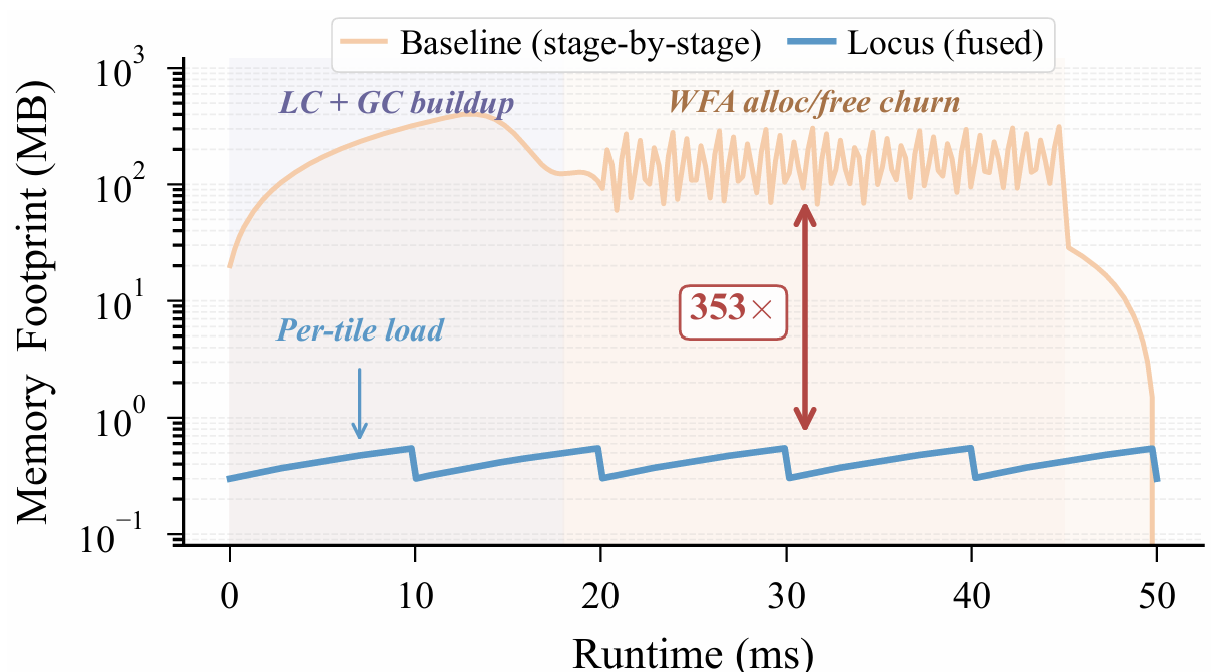
To characterize the temporal behavior of intermediate data traffic, we utilized Minigraph to track the memory footprint. Figure 3 shows the resulting trace for a representative $10\mathrm{Kbp}$ read. The baseline exhibits a pronounced sawtooth pattern: memory grows as each stage accumulates intermediate results, partially drops when some buffers are released, and rises again as subsequent stages allocate new working sets. Wavefront Alignment (WFA) contributes the largest spikes, since each gap induces a buffer scaling with $\bar{L}_g^2$ and multiple allocations overlap in time. Although the peak working set is only $\sim 60\mathrm{MB}$, the instantaneous active data is much smaller. Only one or a few WFA buffers are live at any moment. In contrast, cumulative allocation (i.e., the integral over all alloc/free events) reaches $\sim 1.2\mathrm{GB}$, a $20\times$ amplification over the peak footprint. This discrepancy directly motivates fusion: by retaining intermediate results on-chip and reusing the WFA scratchpad across gaps, cumulative DRAM traffic can be reduced toward the peak working-set bound.

This inefficiency is further exacerbated by bubble regions. As described in Section II-A, linear regions produce long, contiguous local chains that traverse chaining and alignment with minimal graph interaction. In contrast, bubble regions fragment chains across alternative allele segments, forcing repeated shortest-$k$ path queries and repeated DRAM fetches of partitioned subgraphs. Moreover, bubble nodes have an average length of $\sim 108\mathrm{bp}$, which increases gap sizes and further inflates WFA buffer demands. As a result, bubble regions dominate DRAM traffic despite accounting for only $40\%$ of nodes. This imbalance motivates the bubble-aware partitioning strategy in Section III-B.

Fig. 3: Memory footprints of Minigraph and Locus.

III. VARIATION-AWARE PANGENOME GRAPH PARTITIONING

A. DRAM Traffic Modeling

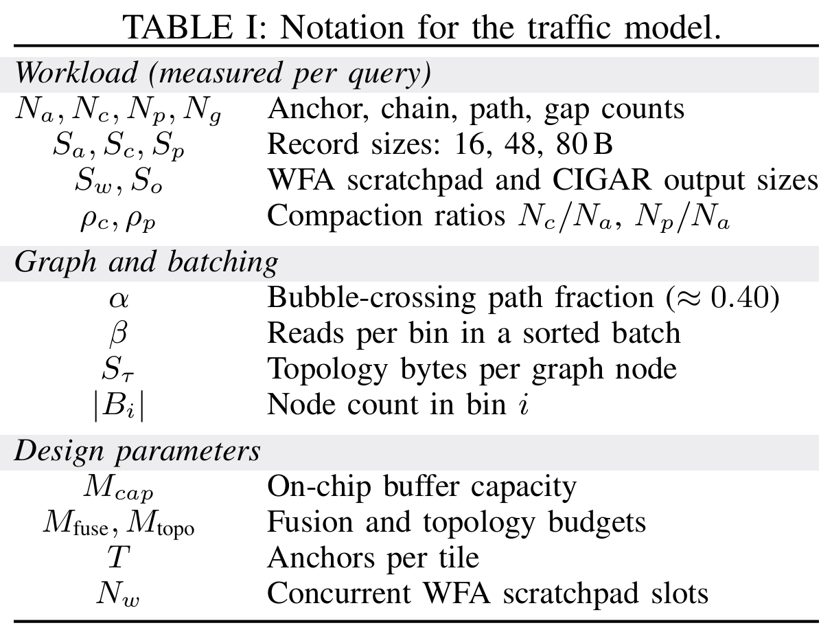
We derive DRAM traffic for baseline and fused execution from the same three-stage pipeline (LC, GC, AL). Table I lists the symbols; record sizes are taken directly from the Minigraph source.

Baseline. For traditional stage-by-stage S2G mapping, each stage reads the input from DRAM and writes the output back. Given a query that produces $N_{a}$ anchors, the per-stage DRAM traffic is:

$\begin{array}{rl} D_{\mathrm{LC}} &= N_aS_a + N_cS_c \\ D_{\mathrm{GC}} &= N_cS_c + \alpha N_pS_\tau +N_pS_p \\ D_{\mathrm{AL}} &= N_pS_p + N_gS_w + N_gS_o \end{array} \quad (4)$

Here, $D_{\mathrm{LC}}$ loads the full anchor set and writes chain descriptors. $D_{\mathrm{GC}}$ reads the chains back, fetches the subgraph (edge lists and node lengths) for the $\alpha \approx 0.40$ fraction of paths that cross bubble regions, and writes graph-chain paths. $D_{\mathrm{AL}}$ reads the paths, allocates and discards a WFA scratchpad for each of the $N_{g}$ gaps, and writes the CIGAR output. The total baseline traffic is the sum $D_{\mathrm{base}} = D_{\mathrm{LC}} + D_{\mathrm{GC}} + D_{\mathrm{AL}}$. The chain term $N_{c}S_{c}$ appears in both $D_{\mathrm{LC}}$ (written) and $D_{\mathrm{GC}}$ (read back), and the path term $N_{p}S_{p}$ appears in both $D_{\mathrm{GC}}$ and $D_{\mathrm{AL}}$. These are the stage-to-stage round trips that fusion eliminates. For long reads $L\geq 10\mathrm{Kbp}$ the WFA scratchpad term $N_{g}S_{w}$ dominates $D_{\mathrm{base}}$ exceeding $86\%$ of total traffic.

Fused Execution. With our proposed stage fusion, each read’s anchors are partitioned into tiles of size $T$ and each tile proceeds through $\mathrm{LC}\to \mathrm{GC}\to \mathrm{AL}$ within an on-chip buffer of capacity $M_{\mathrm{fuse}}$. Chain descriptors, path headers, and WFA scratchpad data are retained across stage boundaries and therefore never traverse DRAM. For the topology term, the host groups reads by their mapped bin and submits them to Locus one bin at a time, allowing the subgraph data of each bin (i.e., vertex sequences and adjacency lists) to be loaded once and reused by all $\beta$ reads in that batch. The resulting per-query traffic becomes:

$D_{\mathrm{fuse}} = \underbrace{N_aS_a}_{\mathrm{anchors}} + \underbrace{\frac{\alpha N_pS_\tau}{\beta}}_{\mathrm{topology}/\beta} + \underbrace{N_gS_o}_{\mathrm{CIGAR}} \quad (5)$

The three terms represent the initial anchor load, the partitioned subgraph data (edge lists, segment identifiers, and node lengths), and the alignment output. Note that $T$ does not appear in $D_{\mathrm{fuse}}$, because once the tile fits on the chip, making it larger or smaller changes neither the DRAM traffic nor the subgraph partition. Tile size matters only for on-chip throughput and appears in the capacity bound below.

On-chip buffer capacity bound. The on-chip buffer must hold the current tile’s anchors, its in-flight intermediates, and partitioned subgraphs:

$TS_{a} + \rho_{c}TS_{c} + \rho_{p}TS_{p} + N_{w}S_{w} + |B_{i}| \cdot S_{\tau} \leq M_{cap} \quad (6)$

where $TS_{a}$ is the tile’s anchor buffer, $\rho_{c}TS_{c}$ and $\rho_{p}TS_{p}$ use the measured compaction ratios $\rho_{c} = N_{c} / N_{a}$ and $\rho_{p} = N_{p} / N_{a}$ to constrain the chain and path buffer sizes proportionally to $T$. $N_{w}S_{w}$ is the WFA scratchpad for $N_{w}$ concurrent gap alignments, and $|B_{i}|$ is the subgraph size.

DRAM access reduction. Compared with stage-by-stage S2G mapping, our proposed fusion strategy has a DRAM-traffic reduction of $R = \frac{D_{\mathrm{base}}}{D_{\mathrm{fuse}}}$. For long reads, $N_{g}S_{w}$ dominates the numerator and $N_{a}S_{a}$ dominates the denominator, so $R$ is limited by the anchor-load floor. Based on our results, $R$ ranges from $24\times$ for 100 bp short reads to $27\times$ for 10 Kbp long reads (Section V-E). The graph partitioning contributes an additional $10\%$ reduction for batches with $\beta \approx 10-50$, which is the typical range for $30\times$ whole-genome coverage.

B. Proposed Pangenome Graph Partitioning

Although many efforts [2], [4], [5], [7], [8] have been made to accelerate genome graph analysis, existing approaches predominantly focus on algorithmic optimizations for computation or instruction-level parallelism, without fully exploiting the data parallelism of pangenome graphs during data partitioning. For example, TALCO [7] exploits the convergence property of traceback pointers in sequence alignment to enable tile-based parallel computation, effectively reducing redundant memory accesses; however, it targets dynamic programming matrices instead of pangenome graphs. GenDP [4] tiles the intra-cell data-flow graph of DP objective functions onto fixed-structure compute units, optimizing operator-level mapping within a single DP cell. SeGraM [2] applies a divide-and-conquer windowing strategy over the two-dimensional alignment space formed by a linearized subgraph and a query read to bound on-chip memory usage, but truncates long-range structural variant edges beyond a fixed hop limit, leaving bubble integrity unaddressed at the graph partitioning level.

In addition, unlike traditional graphs (e.g., social networks, recommendation networks) that typically follow a power-law distribution, pangenome graphs have a near-linear topology with localized bubble structures. Specifically, the vast majority of nodes form long, unbranched sequence chains, while the graph branches into alternative paths to represent genetic variants, represented as bubbles, and later rejoins the main path. Such graph patterns introduce two conflicting demands for tile-based on-chip execution. First, the linear sequence regions are amenable to simple, contiguous memory allocation and exhibit high spatial locality; splitting them arbitrarily incurs negligible communication overhead. In contrast, bubble regions create long-range dependencies between their entry and exit nodes; any partition boundary that cuts through a bubble induces cross-tile communication among its alternative paths, thereby reducing on-chip reuse and increasing off-chip DRAM traffic. The challenge is further compounded by the wide variation in bubble size, from single-nucleotide polymorphisms spanning only a few base pairs to structural variants spanning thousands, which makes uniform partitioning strategies ineffective. These characteristics collectively motivate a bubble-aware partitioning scheme that (1) preserves bubbles as indivisible units, (2) considers bubble size for tiling decisions, and (3) dynamically balances tile utilization rather than enforcing a fixed assignment.

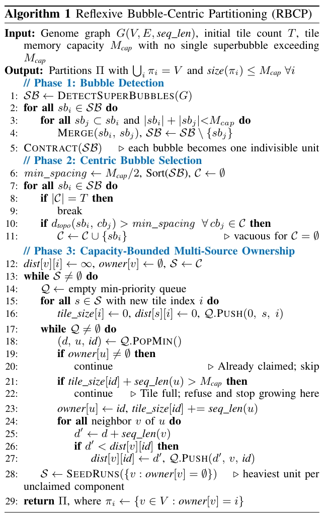
Based on the DRAM access model, we propose Reflexive Bubble-Centric Partitioning (RBCP), a new partitioning algorithm that exploits the unique topology of pangenome graphs by distinguishing linear sequence regions from variant-induced bubble regions. The goal of RBCP is to maximize on-chip data locality while minimizing communication caused by long-range dependencies. Overall, RBCP proceeds in three stages. First, it characterizes the graph topology by detecting all bubble structures. Second, it selects tile centers by anchoring each partition around a large representative bubble. Third, it assigns every remaining node to exactly one tile using a distance-driven ownership mechanism. As shown in Algorithm 1, RBCP adopts the superbubble detection algorithm 31 to identify all bubbles and collapse each of them into a single supernode, ensuring that no variation region is split across tiles. It then selects multiple central bubbles as partition centers to enable parallel partitioning, spacing them at least $M_{cap}/2$ apart so that neighboring tiles do not compete for the same region. Finally, RBCP performs a capacity-bounded multi-source Dijkstra expansion [52] from all central bubble supernodes simultaneously, following edges in both directions. Each unit is claimed by the nearest center that still has room for it; a center whose tile would overflow $M_{cap}$ refuses the unit and stops growing in that direction, which keeps every tile both within capacity and connected. Because a refused unit must remain eligible for its second-nearest center, RBCP tracks the expansion distance per center rather than globally. A unit that no existing tile can accept becomes the seed of a new tile, so the partitioning covers the whole graph and $|\Pi |$ follows from $M_{cap}$ rather than being fixed in advance. Each round seeds one new tile per connected component of the still-unclaimed subgraph, so the unclaimed set strictly shrinks and the loop terminates. Partitioning is a one-time offline step costing $O(K(|V| + |E|)\log |V|)$; on the near-linear pangenome topology only a constant number of centers lie within $M_{cap}$ of any node, so the observed cost approaches that of a single multi-source expansion. RBCP assumes that no single contracted bubble exceeds $M_{cap}$: the merge rule in Phase 1 never creates one, but a primitive superbubble larger than $M_{cap}$ needs to be decomposed into its alternative paths, the only case that breaks the bubble integrity.

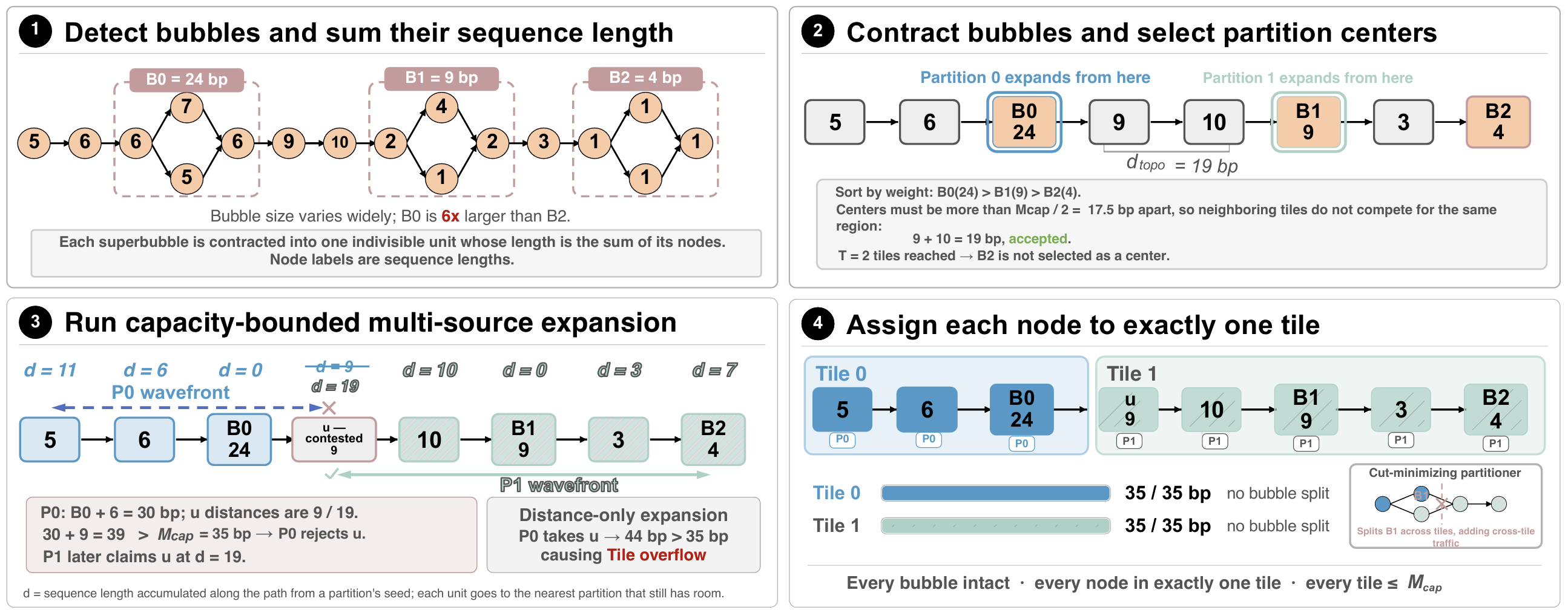
Fig. 4: Walkthrough of RBCP on an eight-unit example with $M_{cap} = 35$ bp.

Figure 4 walks through the three phases of Algorithm 1 on an eight-unit example with $M_{cap} = 35$ bp. Panel 1 shows superbubble detection, which identifies three bubbles and weights each by the sequence length it spans: $24$ bp for $B_{0}$, $9$ bp for $B_{1}$, and $4$ bp for $B_{2}$. Panel 2 contracts each bubble into one indivisible unit, giving the chain $5 \rightarrow 6 \rightarrow B_{0}(24) \rightarrow u(9) \rightarrow 10 \rightarrow B_{1}(9) \rightarrow 3 \rightarrow B_{2}(4)$ of $70$ bp in total, and takes the two largest bubbles as the centers of Partition 0 and Partition 1; they lie $d_{topo} = 19$ bp apart, satisfying the $M_{cap} / 2 = 17.5$ bp spacing rule, while $B_{2}$ is left unselected because the tile budget is already met. Panel 3 shows the expansion, in which each partition claims the nearest unclaimed unit and distance is the sequence length accumulated along the path from its center. The contested unit $u$ lies $9$ bp from Partition 0 and $19$ bp from Partition 1, but Partition 0 already holds $B_{0}$ and the adjacent $6$ bp unit for a total of $30$ bp, so $30 + 9 = 39$ bp would exceed the capacity. Partition 0 therefore refuses $u$ and admits the $5$ bp unit at its far end instead, closing at $35$ bp, and Partition 1 claims $u$ when its own expansion reaches it. Panel 4 gives the result: two tiles of exactly $35$ bp with all three bubbles intact. Had the expansion used distance alone, Partition 0 would have taken $u$ and closed at $44$ bp, overflowing the tile it is meant to fit.

IV. LOCUS ACCELERATOR ARCHITECTURE

Beyond graph partitioning, fusing S2G mapping stages imposes two additional hardware requirements: the on-chip buffer must retain intermediate data across mapping stages, and it must store the graph data of the current partition so that multiple reads can reuse it without repeated DRAM accesses.

A. Proposed Locus Architecture

Figure 5 provides an overview of the proposed Locus architecture. The accelerator comprises a $12 \times 12$ reconfigurable PE array, a two-level memory hierarchy (global buffer and local scratchpad), a Graph Path Finder (GPF) engine, a Traceback Engine, and a Range Maximum Query (RMQ) engine [44], [45].

Global buffer organization. The global buffer (GLB) is divided into four logical banks that can support both intermediate data reuse and graph reuse. The banks support intermediate data exchanged across fused stages: the Anchor Bank stores seed anchors consumed by linear chaining, the Intermediate Result (IR) Bank maintains chaining scores and traceback pointers passed to graph chaining and alignment, and the Sequence Bank stores packed DNA subsequences for base-level comparison. In addition, banks store graph structures shared across reads: the Graph Topology Bank caches vertex sequences and adjacency lists for the currently active partition bin. This bank is double-buffered, allowing the next bin’s data to be prefetched while the current bin is being processed. The banks are divided to reflect the structural invariant of $\alpha \approx 0.40$: approximately $60\%$ of the GLB capacity is assigned to the fusion working set for dataflow parallelism, and $40\%$ is assigned to shared subgraph data for data parallelism. This static partitioning avoids runtime arbitration while matching the expected workload distribution implied by its graph structure.

Control and mode switching. The main controller orchestrates tile execution through a three-phase FSM (Load, Execute, Writeback) and manages transitions between pipeline stages. The controller incorporates a Tile Prefetch Engine (TPE) that implements the data parallelism mechanism through three functions: (1) a four-entry tile queue that buffers pending tile metadata from the host, (2) a prefetch trigger that initiates DMA transfers for the next bin’s vertex sequences and adjacency lists into the inactive double-buffer bank, and (3) buffer swap control that toggles between double-buffered banks upon tile completion. The host side determines the bin (i.e., the partition containing the most anchors during tile batching). TPE receives this bin ID along with the next vertex address and coordinates prefetch timing to hide memory latency behind computation. Switching between chaining and alignment modes requires reconfiguring PE datapath multiplexers and interconnection topology. The transition protocol drains in-flight operations ($2$ cycles), broadcasts mode configuration to all PEs ($1$ cycle), and reconfigures GLB arbitration (overlapped). Total transition latency is $3$ cycles per mode switch, amortized across thousands of operations per tile.

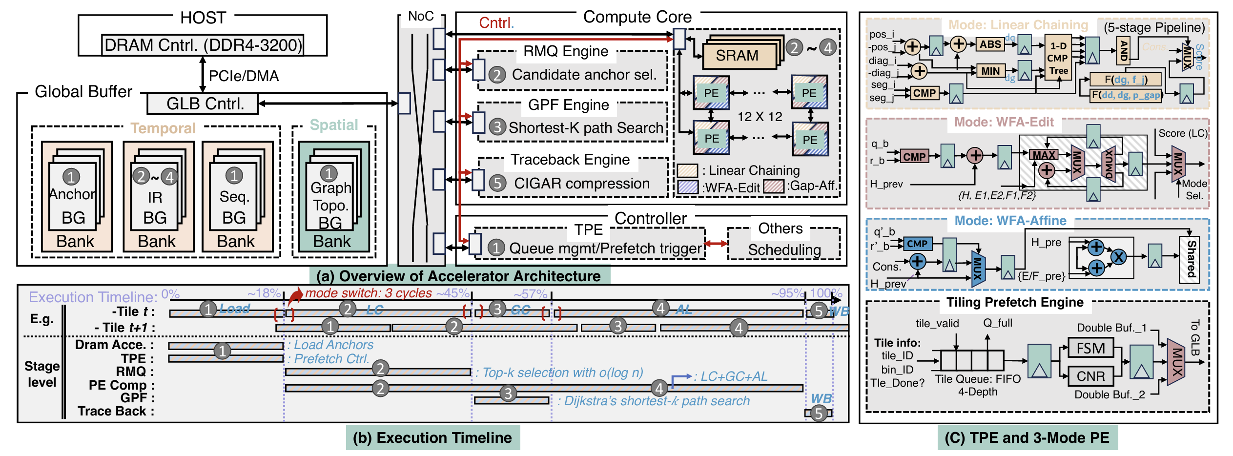
Fig. 5: Proposed Locus Accelerator Microarchitecture: (a) overview of the proposed accelerator architecture, (b) execution time breakdown, and (c) tile prefetch engine and reconfigurable PE.

B. Reconfigurable PE Array

Dataflow parallelism through fusion requires executing linear chaining, graph chaining, and alignment on unified hardware; if each stage required dedicated compute units, intermediate data would traverse separate buffers and reuse would be lost. The Locus PE array addresses this through mode-based reconfiguration: each PE contains shared arithmetic units (adders, comparators, max-selectors) that are dynamically repurposed across three operating modes. Mode-specific datapaths are power-gated when inactive.

Mode 1: Chaining. This mode is used during linear chaining, which connects seed anchors within the same graph segment into co-linear chains, and is reused during graph chaining to score cross-segment transitions once the GPF engine supplies the graph-path distance. The input to this mode is a pair of anchors $(a_{j},a_{i})$ from the Anchor Bank, where each anchor $a_{i}$ is broadcast to all PEs, which encodes query position, reference position, and segment ID. Each PE holds a distinct predecessor anchor candidate $a_{j}$. The PE datapath computes the chaining score defined in Equation 1.

It computes the coordinate differences, evaluating the gap penalty through a $\log_2$ lookup table, and produces a scalar score as output. Since the chaining recurrence requires the best-scoring predecessor among all valid candidates, the RMQ engine narrows the candidate set in $O(\log n)$ time using a segment tree before the PE array evaluates the surviving pairs, so no inter-PE reduction is required. The winning score and predecessor index are written to the IR Bank in the GLB. In this mode, PEs operate independently with no inter-PE data exchange. The PE array processes one anchor $a_{i}$ per cycle across all candidates in parallel.

Mode 2: Wavefront alignment (affine gaps). This mode is used during the alignment stage for base-level sequence comparison with affine gap penalty. Each PE handles one diagonal of the wavefront alignment matrix. The input to the PE array is a pair of sequences: the query subsequence from the Sequence Bank and the reference path from the IR Bank. Each PE reads the five wavefront components (the match state and two affine gap states per direction) from its local scratchpad, receives boundary scores from neighboring PEs, computes the furthest-reaching offsets for the next score, and writes the results back to the scratchpad. Specifically, insertion scores flow from left to right between horizontally adjacent PEs, deletion scores flow from right to left, and match scores flow diagonally. Each PE performs $9$ scratchpad reads and a $5$-way maximum selection per cycle. The output is a completed alignment score and a set of traceback pointers stored in the scratchpad, which the traceback engine later compresses into a CIGAR string. This mode is used for the final base-level alignment where accuracy requires distinguishing gap-open and gap-extend penalties.

Mode 3: Wavefront alignment (edit distance). This mode is a simplified version of Mode 2 used during graph chaining to verify candidate paths through bubble regions. Each PE handles one diagonal of the edit-distance wavefront. The input and PE-to-PE data flow are the same as Mode 2, but the scoring uses a uniform cost of $+1$ for all edit operations instead of separate gap-open and gap-extend penalties. This simplification reduces the computation from five DP matrices to three and from $9$ scratchpad reads per cycle to $3$. The output is an edit-distance score used to evaluate whether a candidate path through a bubble is valid. Mode 3 shares the same physical interconnect as Mode 2; the PE selects between affine and edit-distance scoring through a multiplexer controlled by the mode register.

Local scratchpad. The PE array connects to a local scratchpad that stores wavefront DP matrices during alignment. Unlike GLB data that persists across tiles, scratchpad contents are transient within a single alignment task. The scratchpad is organized into five logical regions corresponding to WFA matrix types. Placing DP matrices in local scratchpad rather than GLB reduces access latency from $3$ cycles to $1$ cycle, critical for sustaining PE throughput during the memoryintensive wavefront computation.

C. Graph Path Finder Engine

Graph chaining extends linear chains across segment boundaries by finding shortest paths through the pangenome graph. When a chain on segment $s_i$ must connect to a chain on segment $s_j$, the GPF engine determines whether a valid path exists and computes its distance. This information scores cross-segment transitions and identifies intermediate vertices for bridging.

The GPF implements a priority-queue-based shortest-path search [53]. For each query, the engine explores paths from source to destination vertex, maintaining candidates ordered by cumulative distance. Search terminates once the $k$ shortest source-to-destination paths have been extracted (default $k = 4$, matching the shortest-$k$ query of Section II-B) or when the distance exceeds a threshold (typically $2\times$ the coordinate-based estimate). The GPF comprises four components: (1) a binary-heap priority queue with hardware-managed insert ($2$ cycles) and extract-min ($3$ cycles) supporting $256$ entries; (2) a distance table recording visited vertices and optimal costs to prevent redundant exploration; (3) an arc cache buffering recently accessed adjacency lists; and (4) a path reconstruction unit that traces back through the distance table to emit the vertex sequence. The engine operates concurrently with PE-array execution: while the PE array computes linear chaining for anchor batch $b + 1$, the GPF processes graph queries from batch $b$. This overlap hides GPF latency for tiles where graph chaining is not on the critical path. For bubble-dense regions where GPF becomes the bottleneck, the controller throttles PE throughput to maintain correct sequencing.

D. Traceback Engine

After the PE array completes wavefront alignment for each gap, the traceback engine reads the score matrix and direction pointers from the local scratchpad, walks backward along the optimal alignment path, and compresses the result into a CIGAR string. The output is written to the IR Bank as the final mapping result. The traceback engine operates concurrently with the next tile’s load phase, so its latency is hidden behind DRAM prefetch for the subsequent tile.

Fig. 6: Proposed dataflow mapping.

E. Proposed Mapping and Dataflow

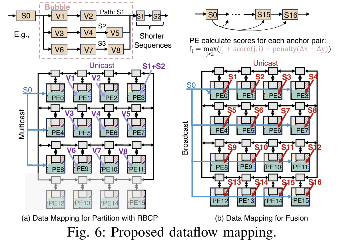
To mitigate long-range graph dependencies and resource underutilization in pangenome graphs, we propose a complementary dataflow strategy that co-locates bubble-interior nodes on adjacent PEs and uses sequential nodes to fill the remaining compute capacity for better workload balance. The key insight is that RBCP already identifies each bubble $(s_i, t_i)$ and its interior nodes during Phase 1 (Algorithm 1). We leverage this information in an offline preprocessing step to construct a bubble-topology prefetching table (BPT), a compact static mapping that assigns each bubble to a contiguous block of PE rows. Because sequential nodes are typically shorter, they can then be used to fill remaining capacity with negligible overhead. Specifically, the BPT maps each alternative path within a bubble to a dedicated PE row, while the entry and sink nodes are multicast and collected across rows to avoid redundant computation. Within each row, intermediate DP scores are forwarded directly between adjacent PEs through the register file. Since alternative paths within a bubble vary in both node count and per-node sequence length, shorter paths inevitably leave their assigned PE rows idle before longer paths complete. Sequential nodes that carry no dependence on the in-flight bubble, such as those from other reads batched onto the same tile, naturally complement this imbalance: because they have shorter average sequence lengths than bubble-interior nodes, they can be scheduled into the remaining compute budget of underutilized PE rows and executed in parallel with longer bubble paths. Overall, RBCP preserves bubble integrity at the macro level through tile formation, while the BPT co-locates bubble paths onto dedicated PE rows and fills idle cycles with sequential nodes at the micro level, thereby improving PE utilization during bubble traversal.

As illustrated in Figure 6(a), consider a bubble with three alternative paths $\{S1, S2, S3\}$ traversing interior nodes $\{V1, ..., V8\}$. The entry node $S0$ is multicast to all PE rows simultaneously. Path $S1$ is assigned to PE row $0$ (PE0-PE3), path $S2$ to row $1$ (PE4-PE7), and path $S3$ to row $2$ (PE8-PE11), each processing its interior nodes sequentially with register-level forwarding. The sink nodes are assigned only once upon path convergence. Since paths $S1$ and $S2$ are shorter than $S3$, PE rows $0$ and $1$ finish early. The subsequent sequential nodes (e.g., $S1 \rightarrow S2$ in the linear region) are unicast to these idle rows, keeping all PEs active until the bubble is fully resolved. Supporting these modes requires reconfiguring PE-to-PE connectivity to match algorithmic data dependencies. We design the dataflow as shown in Figure 6(b). Chaining requires collecting a global maximum from distributed local scores in each PE, while WFA requires exchanging values between neighboring diagonals. For chaining, the RMQ engine performs coarse candidate selection using a segment tree [44], [45] in $O(\log n)$ time, reducing the candidate set from all anchor pairs to a filtered subset. Since RMQ handles selection, the PE array evaluates only the selected $(i,j)$ pair; anchor $i$ is broadcast to all PEs, but no inter-PE reduction is needed. For wavefront alignment, each PE handles one diagonal and exchanges boundary values with its horizontal neighbors: $E$ matrices flow rightward and $F$ matrices flow leftward, matching the cross-diagonal dependencies. This is set by the mode register and reconfigured in the same cycle as the datapath multiplexers.

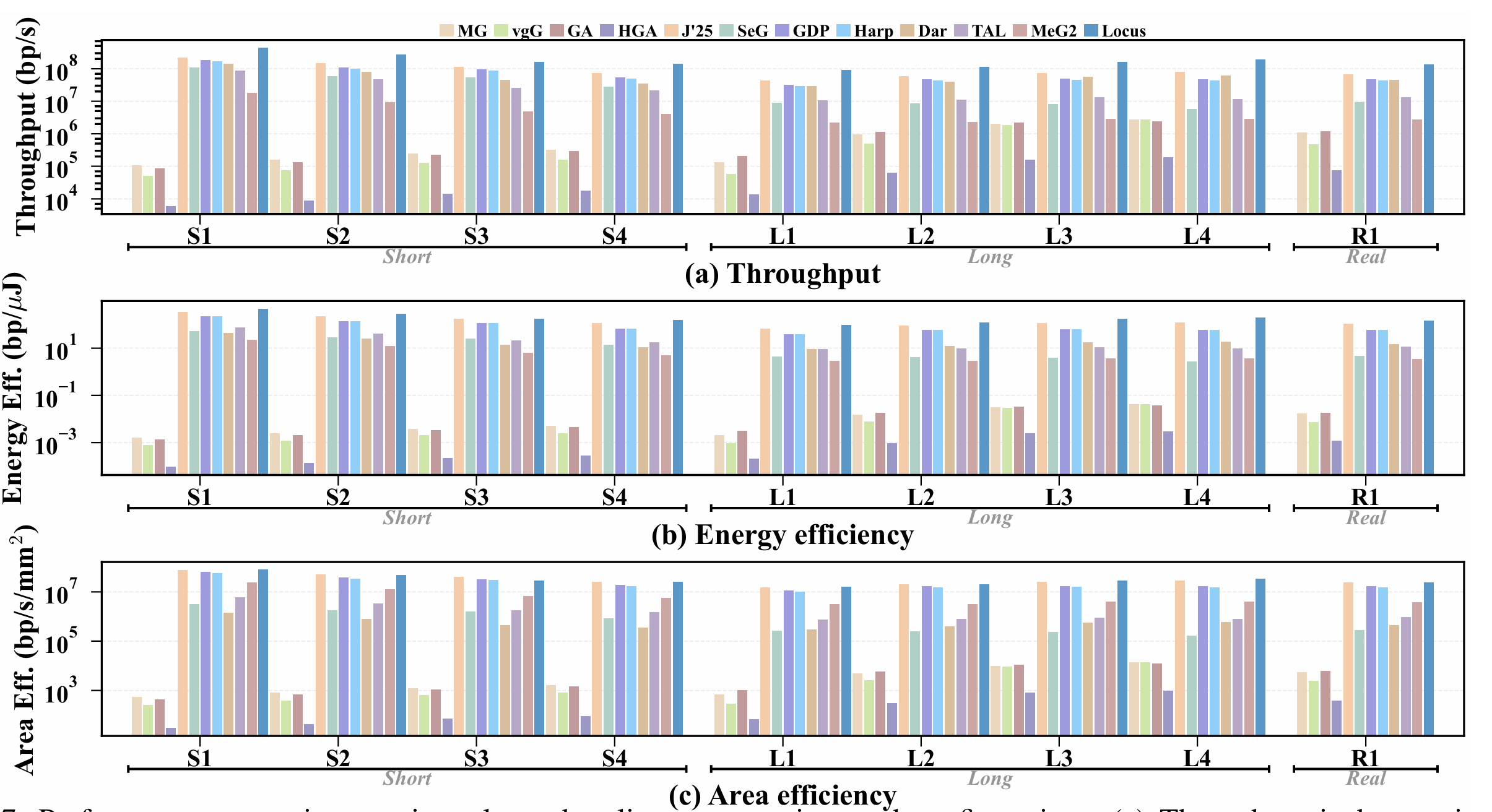
Fig. 7: Performance comparison against eleven baselines across nine read configurations. (a) Throughput in base pairs per second. (b) Energy efficiency in base pairs per microjoule. (c) Area efficiency in base pairs per second per $\mathrm{mm}^2$. All axes are logarithmic; ASIC and PIM results are normalized to $28~\mathrm{nm}$.

V. EVALUATION

A. Experimental Setup

Hardware Implementation. We synthesized the Locus RTL design using Synopsys Design Compiler with SAED $28~\mathrm{nm}$ technology library under the worst-case PVT corner at $1\mathrm{GHz}$. Power estimation uses Synopsys PrimePower. Area results are extracted from placed-and-routed designs using Synopsys IC Compiler II [54]. For DRAM timing, we integrate with Ramulator [55] configured as DDR4-3200 ($25.6\mathrm{GB/s}$ peak bandwidth). Throughput and energy are obtained from cycle-accurate RTL simulation of the complete design; Ramulator supplies DRAM timing, and PrimePower derives switching activity from the resulting value-change traces. The global buffer uses single-cycle SRAM banks.

Datasets. We generate synthetic query sequences from human autosomes (chromosomes 1 through 22) of the GRCh38 human reference assembly [1], following the methodology established by prior pangenome accelerator studies [2], [5]. To evaluate scalability across read lengths, we construct nine configurations spanning four short-read lengths and four long-read lengths, plus one real-data experiment. For short reads, we employ ART [56] with the HiSeq 2500 profile [57] to generate $100~\mathrm{bp}$, $150~\mathrm{bp}$, $250~\mathrm{bp}$, and $300~\mathrm{bp}$ reads at a $0.1\%$ substitution error rate. For long reads, we use PBSIM3 [58] with the ERRHMM-SEQUEL model to simulate $1~\mathrm{Kbp}$, $10~\mathrm{Kbp}$, $50~\mathrm{Kbp}$, and $100~\mathrm{Kbp}$ reads at a $1\%$ error rate. PBSIM3 generates reads to a target coverage, so counts vary slightly by configuration; Table II reports the exact number of reads in each set. Both simulators provide ground-truth alignments in MAF format for precision and recall validation. In addition, we include $10,000$ subsampled PacBio HiFi reads ($\sim 15~\mathrm{Kbp}$ average length, $\sim 0.1\%$ error rate) from the HG002 (NA24385) sample provided by the Genome in a Bottle Consortium [59], representing real sequencing data with authentic error profiles and read length distributions. For the pangenome reference, we use the GRCh38 graph (v1.1) from the Human Pangenome Reference Consortium (HPRC) [9], [27], which incorporates 94 diverse haplotypes spanning 3.1 billion base pairs.

Baselines. We compare Locus against eleven baselines spanning four computing platforms. For software baselines, we evaluate three CPU-based tools: GraphAligner [33], Minigraph [26], and vg Giraffe [35]; and one GPU-based tool: HGA [60] running on NVIDIA A100 GPUs. All software tools are compiled with optimization flags and executed on the same server with 500 GB of RAM. For hardware baselines, we compare against six ASIC accelerators: Darwin [6], SeGraM [2], GenDP [4], Harp [5], TALCO [7], and JSsCC’25 [3]. We also include one processing-in-memory design, MeG2 [8]. To ensure fair comparison, all ASIC and PIM results are normalized to $28\mathrm{nm}$ using standard technology scaling factors [61]. For baselines that report results at different read lengths or error rates, we compare at the closest available configuration.

B. Performance Comparison

Figure 7 compares Locus with all eleven baselines across the nine configurations of Section V-A; panels (a)-(c) report throughput, energy efficiency, and area efficiency on logarithmic axes. Because the hardware baselines accelerate different subsets of the S2G pipeline, we credit each with zero cost for the stages it does not implement. Since a design covering only part of the pipeline can be no faster end to end than the stages it covers, these figures are upper bounds, and the margins we report are correspondingly lower bounds. Because Locus covers linear chaining, graph chaining, and alignment, its figure spans strictly more work per mapped base than the partial-coverage designs. Locus sustains 96-471 Mbp/s and delivers the highest throughput at every configuration. JSsCC’25 is the strongest baseline in all three metrics; Locus exceeds it by $2.1\times$, $1.2\times$, and $1.1\times$ in geometric mean, with the throughput margin spanning $1.5 - 2.6\times$. The margin reaches $2.9 - 9.6\times$ over the other ASICs, $44\times$ over MeG2, and 390-$700\times$ over the CPU mappers.

The baselines themselves show that fusion, not per-stage compute density, dominates end-to-end throughput. GenDP and JSsCC’25 accelerate the same two stages and differ mainly in that JSsCC’25 retains part of the intermediate data on chip between them; JSsCC’25 leads GenDP at all nine configurations by $1.4\times$. Single-stage designs (Darwin, TALCO) and those omitting alignment (Harp) trail further, since their uncovered stages still exchange results through DRAM. Locus extends fusion to the complete LC-GC-AL chain, so its advantage grows with the volume of intermediate data: the margin over JSsCC’25 rises from $1.9\times$ on short reads to $2.3\times$ on long reads, peaking at $2.6\times$ at $100\mathrm{Kbp}$ and tracking the quadratic growth of the WFA scratchpad with gap length (Section II-C). The margin is narrower at $250\mathrm{bp}$, where Locus holds $1.5\times$ throughput but falls to $0.87\times$ and $0.78\times$ of JSsCC’25 in energy and area efficiency; on real HiFi reads it sustains $144\mathrm{Mbp / s}$ at $2.2\times$ the throughput and $1.2\times$ the energy efficiency of JSsCC’25. Fusion is not free in area: at $5.65\mathrm{mm}^2$, Locus is roughly twice the most compact baselines ($2.87\mathrm{mm}^2$ for GenDP and Harp, $2.90\mathrm{mm}^2$ for JSsCC’25), since the global buffer and scratchpad must hold the working set that would otherwise spill to DRAM. Panel (c) shows that in geometric mean the throughput gain more than repays this cost: fusing the full pipeline, rather than widening a single stage, converts the DRAM traffic reduction of Section V-E into throughput and energy efficiency.

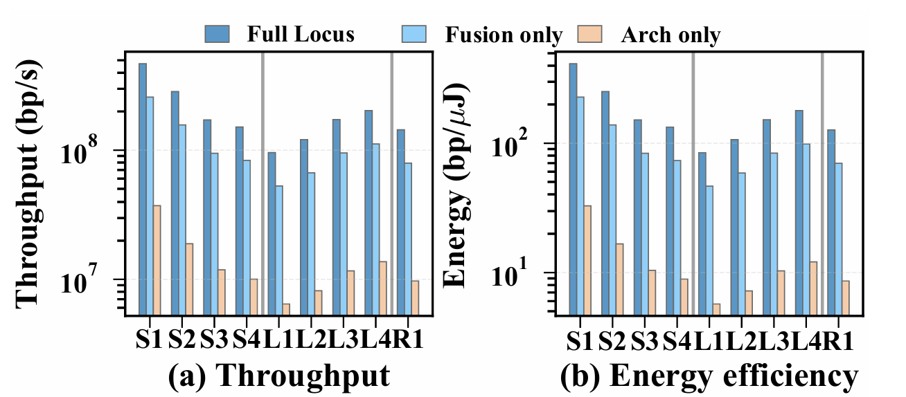
Fig. 8: Ablation study on each Locus technique.

C. Mapping Accuracy

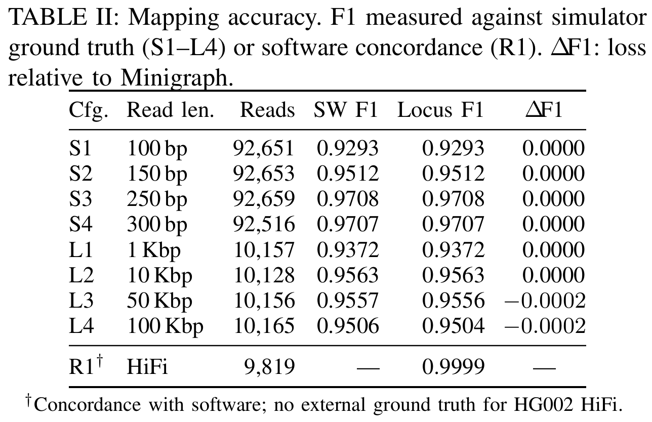
Table II reports mapping accuracy of the Locus functional model against software Minigraph. For simulated reads (S1-L4), F1 is computed against ART/PBSIM3 ground-truth alignments with $200\mathrm{bp}$ position tolerance. Across all eight simulated configurations, Locus achieves identical F1 to software for reads up to $10\mathrm{Kbp}$ and differs by at most $0.02\%$ for ultra-long reads (50-100 Kbp). The minor divergence on L3-L4 arises from numerical precision in chaining score accumulation over very long anchor sequences. For real HiFi reads (R1), Locus achieves $99.99\%$ concordance with software output. These results confirm that cross-stage fusion and tiled execution preserve mapping accuracy.

D. Ablation Study

Figure 8 shows the contribution of cross-stage fusion and architecture co-design. We evaluate three configurations: full Locus (fusion + architecture), fusion-only (software fusion on baseline hardware), and architecture-only (custom hardware without fusion). Fusion alone achieves $86\%$ DRAM traffic reduction and $55\%$ of full-system throughput. With only accelerator design, it provides no DRAM reduction because each stage still writes intermediate data to DRAM and reads it back for the next stage. The full system achieves $96\%$ DRAM reduction. The additional $10\%$ comes from fetching each graph region once from DRAM and reusing it across multiple reads.

E. DRAM Traffic Reduction Analysis

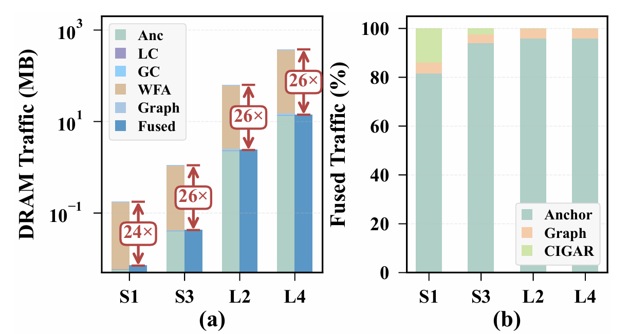
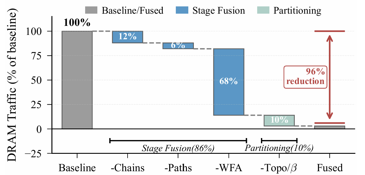
Figure 9 quantifies the DRAM traffic reduction from cross-stage fusion. Panel (a) compares baseline stage-by-stage execution against fused execution across four selected configurations. Baseline traffic is dominated by WFA scratchpad allocation, which accounts for over $85\%$ of total DRAM access for long reads. Fusion eliminates this overhead by keeping WFA buffers on-chip, achieving $24-27\times$ reduction depending on read length. Panel (b) breaks down the fused traffic into three components: anchor input (unavoidable), graph data (vertex sequences and edges, reduced by data parallelism), and CIGAR output (unavoidable). Anchor load dominates because it is the irreducible input to the pipeline; graph data and CIGAR together account for less than $5\%$ of fused traffic. Figure 10 shows the contribution of each optimization. Fusing LC and GC eliminates chain descriptor traffic, reducing DRAM access by $12\%$. Fusing GC and AL eliminates path data traffic, saving another $6\%$. Keeping WFA scratchpad on-chip accounts for the largest reduction at $68\%$, consistent with the quadratic buffer scaling observed in Section II-C. These three components constitute dataflow parallelism, totaling $86\%$. Data parallelism contributes the remaining $10\%$ by loading each partition’s subgraph data once per batch rather than once per read. The final fused traffic is $4\%$ of the baseline.

Fig. 9: DRAM traffic breakdown. (a) Baseline vs fused total. (b) Fused traffic breakdown by component.	Fig. 10: Step-by-step DRAM traffic reduction.

F. Sensitivity Studies

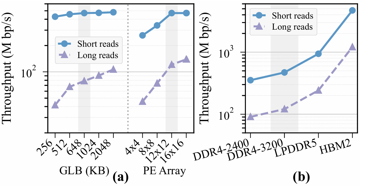
Figure 11 shows throughput sensitivity to three architectural parameters. Panel (a) sweeps GLB capacity (256-2048 KB) and PE array size ($4\times4$ to $16\times16$). For short reads, throughput saturates beyond 648 KB GLB and $12\times12$ PE array—the working set fits on-chip and compute resources exceed memory bandwidth. Long reads continue to benefit from larger GLB ($2.5\times$ gain from 256 KB to 2 MB) and larger PE arrays, reflecting their larger per-query working sets and longer alignment tasks. Panel (b) sweeps DRAM technology from DDR4-2400 to HBM2. Throughput scales nearly linearly with bandwidth: $10\times$ higher bandwidth (25.6 to 256 GB/s) yields $10\times$ higher throughput. This linear scaling confirms that cross-stage fusion shifts the bottleneck from compute to memory bandwidth.

Fig. 11: Throughput sensitivity to (a) GLB and PE array size, and (b) DRAM technology. Gray bands mark Locus’s design point (648 KB, $12\times12$, DDR4-3200)	Fig. 12: Area and power breakdown by component.

G. Area and Power Analysis

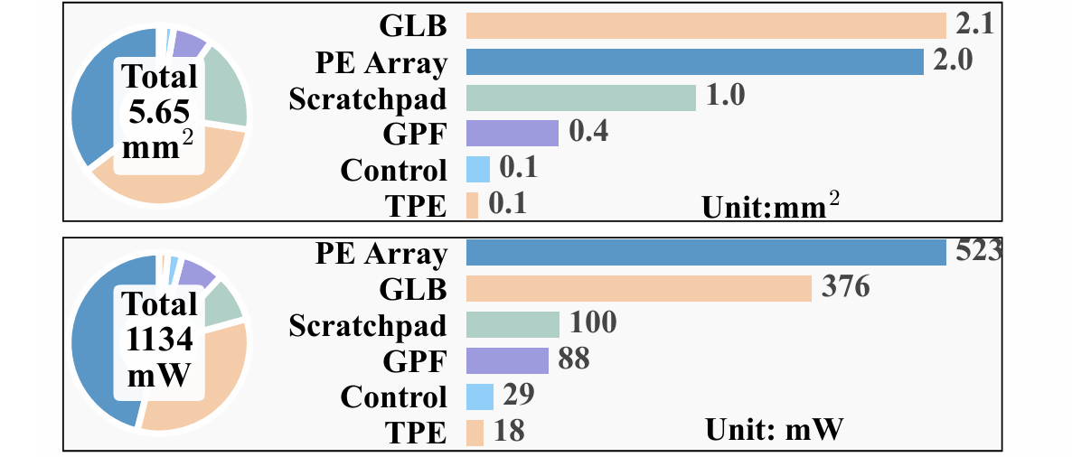
Figure 12 shows the area and power breakdown of Locus synthesized in $28~\mathrm{nm}$ at $1\mathrm{GHz}$: $5.65\mathrm{mm}^2$ and $1.13\mathrm{W}$ in total. The global buffer (GLB) and PE array dominate both, at $72\%$ of area and $79\%$ of power, reflecting the cost of cross-stage fusion—the GLB must hold the fusion working set, and the PE array must sustain throughput across all three pipeline stages. The scratchpad adds $18\%$ of area, the Graph Path Finder only $7\%$ despite its priority-queue-based shortest-path search, and control logic and the TPE together account for under $3\%$.

VI. CONCLUSION

This paper presents Locus, an accelerator for sequence-to-graph mapping on pangenome graphs. We observed that genetic variation encoded as bubbles introduces two key challenges: intermediate data movement between pipeline stages dominates DRAM traffic, and structural irregularity complicates parallelization. To address both, Locus employs a bubble-aware partitioning algorithm that groups variation bubbles while preserving workload balance, and a variation-aware dataflow that fuses multiple mapping stages onto a reconfigurable PE array, eliminating inter-stage DRAM traffic. Evaluated on the HPRC pangenome graph, Locus achieves $2.1\times$ throughput and $1.2\times$ energy efficiency over state-of-the-art accelerators, reducing DRAM traffic by $96\%$, and produces near-identical results to the software Minigraph baseline.

References

[1] V. A. Schneider et al., “The GRCh38 reference genome assembly,” Genome Research, 2017.

[2] D. S. Cali et al., “SeGraM: A universal hardware accelerator for genomic sequence-to-graph and sequence-to-sequence mapping,” in Proceedings of the 49th Annual International Symposium on Computer Architecture, 2022, pp. 638-655.

[3] Y. Zhang, J. Zhu, L. Li, G. Zeng, D. Chen, T. Zhang, Y. Deng, Z. Gong, A. Zhang, Y. Liu et al., “A 28-nm 239-bp/μj agile pangenome analysis accelerator for multi-scheme read mapping,” IEEE Journal of Solid-State Circuits, 2025.

[4] Y. Gu, A. Subramaniyan, T. Dunn, A. Khadem, K.-Y. Chen, S. Paul, M. Vasimuddin, S. Misra, D. Blaauw, S. Narayanasamy et al., “Gendp: A framework of dynamic programming acceleration for genome sequencing analysis,” in Proceedings of the 50th Annual International Symposium on Computer Architecture (ISCA), 2023, pp. 1-15.

[5] Y. Zhang, D. Chen, G. Zeng, J. Zhu, Z. Li, L. Chen, S. Wei, and L. Liu, “Harp: Leveraging quasi-sequential characteristics to accelerate sequence-to-graph mapping of long reads,” in Proceedings of the 29th ACM International Conference on Architectural Support for Programming Languages and Operating Systems, Volume 3 (ASPLOS), 2024, pp. 512-527.

[6] Y. Turakhia, G. Bejerano, and W. J. Dally, “Darwin: A genomics co-processor provides up to 15,000 x acceleration on long read assembly,” ACM SIGPLAN Notices, vol. 53, no. 2, pp. 199-213, 2018.

[7] S. Walia, C. Ye, A. Bera, D. Lodhania, and Y. Turakhia, “Talco: tiling genome sequence alignment using convergence of traceback pointers,” in Proceedings of 2024 IEEE International Symposium on High-Performance Computer Architecture (HPCA). IEEE, 2024, pp. 91-107.

[8] Y. Huang, L. Zheng, H. Liu, Z. Zhou, D. Chen, P. Yao, Q. Wang, X. Liao, and H. Jin, “Meg 2: In-memory acceleration for genome graphs analysis,” in Proceedings of 2023 60th ACM/IEEE Design Automation Conference (DAC). IEEE, 2023, pp. 1-6.

[9] W.-W. Liao et al., “A draft human pangenome reference,” Nature, vol. 617, pp. 312-324, 2023.

[10] J. M. Eizenga, A. M. Novak, J. A. Sibbesen, S. Heumos, A. Ghaffari, G. Hickey, X. Chang, J. D. Seaman, R. Rounthwaite, J. Ebler et al., “Pangenome graphs,” Annual Review of Genomics and Human Genetics, vol. 21, pp. 139-162, 2020.

[11] B. Paten et al., “Genome graphs and the evolution of genome inference,” Genome research, vol. 27, no. 5, pp. 665-676, 2017.

[12] E. Garrison et al., “Variation graph toolkit improves read mapping by representing genetic variation in the reference,” Nature biotechnology, vol. 36, no. 9, pp. 875-879, 2018.

[13] D. Y. Brandt, V. R. Aguiar, B. D. Bitarello, K. Nunes, J. Goudet, and D. Meyer, “Mapping bias overestimates reference allele frequencies at the hla genes in the 1000 genomes project phase i data,” G3: Genes, Genomes, Genetics, vol. 5, no. 5, pp. 931-941, 2015.

[14] D. S. Cali, G. S. Kalsi, Z. Bingöl, C. Firtina, L. Subramanian, J. S. Kim, R. Ausavarungnirun, M. Alser, J. Gomez-Luna, A. Boroumand et al., “Genasm: A high-performance, low-power approximate string matching acceleration framework for genome sequence analysis,” in Proceedings of 2020 53rd Annual IEEE/ACM International Symposium on Microarchitecture (MICRO). IEEE, 2020, pp. 951-966.

[15] D. Fujiki, A. Subramaniyan, T. Zhang, Y. Zeng, R. Das, D. Blaauw, and S. Narayanasamy, “Genax: A genome sequencing accelerator,” in Proceedings of 2018 ACM/IEEE 45th Annual International Symposium on Computer Architecture (ISCA). IEEE, 2018, pp. 69-82.

[16] Y. Cui et al., “A survey of sequence-to-graph mapping algorithms in the pangenome era,” Genome Biology, vol. 26, no. 1, p. 138, 2025.

[17] A. Madhavan et al., “Race logic: A hardware acceleration for dynamic programming algorithms,” ACM SIGARCH Computer Architecture News, vol. 42, no. 3, pp. 517-528, 2014.

[18] G. Karypis and V. Kumar, “Multilevel algorithms for multi-constraint graph partitioning,” in SC’98: Proceedings of the 1998 ACM/IEEE Conference on Supercomputing. IEEE, 1998, pp. 28-28.

[19] P. Sanders and C. Schulz, “High quality graph partitioning,” Graph Partitioning and Graph Clustering, vol. 588, no. 1, pp. 1-17, 2012.

[20] S. Yang, M. Zhang, W. Dong, and D. Li, “Betty: Enabling large-scale gnn training with batch-level graph partitioning,” in Proceedings of the 28th ACM International Conference on Architectural Support for Programming Languages and Operating Systems, Volume 2, 2023, pp. 103-117.

[21] M. F. Faraj and C. Schulz, “Buffered streaming graph partitioning,” ACM Journal of Experimental Algorithmics, vol. 27, pp. 1-26, 2022.

[22] A.-C. Syvänen, “Accessing genetic variation: genotyping single nucleotide polymorphisms,” Nature Reviews Genetics, vol. 2, no. 12, pp. 930-942, 2001.

[23] 1000 Genomes Project Consortium, “A global reference for human genetic variation,” Nature, vol. 526, no. 7571, pp. 68-74, 2015.

[24] S. S. Ho, A. E. Urban, and R. E. Mills, “Structural variation in the sequencing era,” Nature Reviews Genetics, vol. 21, no. 3, pp. 171-189, 2020.

[25] G. Gonnella, N. Niehus, and S. Kurtz, “Gfaziv: flexible and interactive visualization of gfa sequence graphs,” Bioinformatics, vol. 35, no. 16, pp. 2853-2855, 2019.

[26] H. Li, X. Feng, and C. Chu, “The design and construction of reference pangenome graphs with minigraph,” Genome Biology, vol. 21, no. 1, pp. 1-19, 2020.

[27] G. Hickey, J. Monlong, J. Ebler, A. M. Novak, J. M. Eizenga, Y. Gao, T. Marschall, H. Li, and B. Paten, “Pangenome graph construction from genome alignments with minigraph-cactus,” Nature biotechnology, vol. 42, no. 4, pp. 663-673, 2024.

[28] E. Garrison, A. Guarracino, S. Heumos, F. Villani, Z. Bao, L. Tattini, J. Hagmann, S. Vorbrügg, S. Marco-Sola, C. Kubica et al., “Building pangenome graphs,” bioRxiv, 2024.

[29] Z. Guo and H. Wang, “A deep graph neural network-based mechanism for social recommendations,” IEEE Transactions on Industrial Informatics, vol. 17, no. 4, pp. 2776-2783, 2020.

[30] W. Fan, Y. Ma, Q. Li, Y. He, E. Zhao, J. Tang, and D. Yin, “Graph neural networks for social recommendation,” in The world wide web conference, 2019, pp. 417-426.

[31] T. Onodera, K. Sadakane, and T. Shibuya, “Detecting superbubbles in assembly graphs,” in Proceedings of International workshop on algorithms in Bioinformatics (WABI). Springer, 2013, pp. 338-348.

[32] L. Huang, V. Popic, and S. Batzoglou, “Short read alignment with populations of genomes,” Bioinformatics, vol. 29, no. 13, pp. i361-i370, 2013.

[33] M. Rautiainen and T. Marschall, “Graphaligner: rapid and versatile sequence-to-graph alignment,” Genome Biology, vol. 21, no. 1, pp. 1-28, 2020.

[34] J. Sirén, E. Garrison, A. M. Novak, B. Paten, and R. Durbin, “Haplotype-aware graph indexes,” Bioinformatics, vol. 36, no. 2, pp. 400-407, 2020.

[35] J. Sirén, J. Monlong, X. Chang, A. M. Novak, J. M. Eizenga, C. Markello, J. A. Sibbesen, G. Hickey, P.-C. Chang, A. Carroll et al., “Pangenomics enables genotyping of known structural variants in 5202 diverse genomes,” Science, vol. 374, no. 6574, p. abg8871, 2021.

[36] H. Li, “Minimap2: pairwise alignment for nucleotide sequences,” Bioinformatics, vol. 34, no. 18, pp. 3094-3100, 2018.

[37] “Minimap and minimax: fast mapping and de novo assembly for noisy long sequences,” Bioinformatics, vol. 32, no. 14, pp. 2103-2110, 2016.

[38] M. Roberts, W. Hayes, B. R. Hunt, S. M. Mount, and J. A. Yorke, “Reducing storage requirements for biological sequence comparison,” Bioinformatics, vol. 20, no. 18, pp. 3363-3369, 2004.

[39] S. Schleimer, D. S. Wilkerson, and A. Aiken, “Winnowing: local algorithms for document fingerprinting,” in Proceedings of the 2003 ACM SIGMOD international conference on Management of data, 2003, pp. 76-85.

[40] C. Jain, A. Rhie, N. F. Hansen, S. Koren, and A. M. Philippy, “Long-read mapping to repetitive reference sequences using winnowmap2,” Nature methods, vol. 19, no. 6, pp. 705-710, 2022.

[41] H. Zheng, C. Kingsford, and G. Marçais, “Improved design and analysis of practical minimizers,” Bioinformatics, vol. 36, no. Supplement_1, pp. i119-i127, 2020.

[42] D. DeBlasio, F. Gobsoibo, C. Kingsford, and G. Marçais, “Practical universal k-mer sets for minimizer schemes,” in Proceedings of the 10th ACM international conference on bioinformatics, computational biology and health informatics, 2019, pp. 167-176.

[43] G. Marçais, D. Pellow, D. Bork, Y. Orenstein, R. Shamir, and C. Kingsford, “Improving the performance of minimizers and winnowing schemes,” Bioinformatics, vol. 33, no. 14, pp. i110-i117, 2017.

[44] J. Fischer and V. Heun, “A new succinct representation of rmq-information and improvements in the enhanced suffix array,” in Proceedings of International Symposium on Combinatorics, Algorithms, Probabilistic and Experimental Methodologies (ESCAPE). Springer, 2007, pp. 459-470.

[45] M. S. Dvoretskii, “A segment tree based top-k rnq algorithm and its application to the autocomplete problem,” - no. 1 (39), pp. 48-54, 2017.

[46] V. Makinen, A. I. Tomescu, A. Kuosmanen, T. Paavilainen, T. Gagie, and R. Chikhi, “Sparse dynamic programming on DAGs with small width,” ACM Transactions on Algorithms (TALG), vol. 15, no. 2, pp. 1-21, 2019.

[47] C. Jain, H. Zhang, Y. Gao, and S. Aluru, “Co-linear chaining on pangenome graphs,” Algorithms for Molecular Biology, vol. 19, no. 1, p. 12, 2024.

[48] S. Marco-Sola et al., “Fast gap-affine pairwise alignment using the wavefront algorithm,” Bioinformatics, vol. 37, no. 4, pp. 456-463, 2021.

[49] V. Likic, “The needleman-wunsch algorithm for sequence alignment,” Lecture given at the 7th Melbourne Bioinformatics Course, Bio21 Molecular Science and Biotechnology Institute, University of Melbourne, pp. 1-46, 2008.

[50] M. Cavojsky, M. Drozda, and Z. Balogh, “Analysis and experimental evaluation of the needleman-wunsch algorithm for trajectory comparison,” Expert Systems with Applications, vol. 165, p. 114068, 2021.

[51] S. Marco-Sola, J. M. Eizenga, A. Guarracino, B. Paten, E. Garrison, and M. Moreto, “Optimal gap-affine alignment in o (s) space,” Bioinformatics, vol. 39, no. 2, p. btaa074, 2023.

[52] M. Noto and H. Sato, “A method for the shortest path search by extended djkstra algorithm,” in Proceedings of IEEE International Conference on Systems, Man and Cybernetics (SMC), vol. 3. IEEE, 2000, pp. 2316-2320.

[53] E. W. Dijkstra, “A note on two problems in connexion with graphs,” in Edsger Wybe Dijkstra: his life, work, and legacy, 2022, pp. 287-290.

[54] “IC Compiler II: Place & Route Solution - Synopsys - synopsys.com,” https://www.synopsys.com/implementation-and-signoff/physical-implementation/ic-compiler.html.

[55] Y. Kim, W. Yang, and O. Mutlu, “Ramulator: A fast and extensible dram simulator,” IEEE Computer Architecture Letters, vol. 15, no. 1, pp. 45-49, 2015.

[56] W. Huang, L. Li, J. R. Myers, and G. T. Marth, “ART: a next-generation sequencing read simulator,” Bioinformatics, vol. 28, no. 4, pp. 593-594, 2012.

[57] “GEO Accession viewer - ncbi.nlm.nih.gov,” https://www.ncbi.nlm.nih.gov/geo/query/acc.cgi?acc=GSM1182889.

[58] Y. Ono, M. Hamada, and K. Asai, “PBSIM3: a simulator for all types of PacBio and ONT long reads,” NAR Genomics and Bioinformatics, vol. 4, no. 3, 2022.

[59] C. Xiao, J. Zook, S. Trask, S. Sherry, and G. in-a Bottle Consortium, “Giab: Genome reference material development resources for clinical sequencing,” Cancer Research, vol. 74, no. 19, Supplement, pp. 5328-5328, 2014.

[60] Z. Feng and Q. Luo, “Accelerating sequence-to-graph alignment on heterogeneous processors,” in Proceedings of the 50th international conference on parallel processing, 2021, pp. 1-10.

[61] A. Stillmaker and B. Baas, “Scaling equations for the accurate prediction of CMOS device performance from 180 nm to 7 nm,” Integration, the VLSI Journal, vol. 58, pp. 74-81, 2017.