4 PangenomicsBench

PangenomicsBench: A Benchmark Suite and Characterization of Pangenomics

Abstract

Cheaper and more accurate sequencing technologies have led to a large volume of genetic data that poses significant computational challenges and requires novel computing solutions to keep pace. This increased volume has also enabled the use of pangenome graph references, which provide better quality alignments because they can represent variation, but they require new algorithms that are usually slower than their linear counterparts, and exhibit different computational characteristics.

We introduce PangenomicsBench, the first benchmark suite targeting computational pangenomics, with six kernels extracted from popular tools, designed to guide future research in optimizing pangenomics software and hardware acceleration. We also perform in-depth workload characterization of our kernels. Our analysis reveals the following key insights: (a) Graph alignment algorithms are limited by control complexity rather than memory access to the reference graph, as they process small, cache-friendly subgraphs. (b) Graph construction introduces computational patterns different from linear genomics like stochastic gradient descent. (c) Pangenomic mapping algorithms are highly sensitive to reference graph structures. (d) There are opportunities for optimizing existing software.

I. INTRODUCTION

Genome sequencing is a key component of precision health, allowing us to tailor treatment to individuals based on their genetics. A decade ago, it cost $10 million to sequence a single genome, but today we can do the same for less than $1000 [1]. This has resulted in a large volume of sequencing data and assembled genomes, which have given rise to the new subfield of computational pangenomics. A pangenome is a set of multiple genomes which can be represented with a unified graph data structure and can be used to make comparisons within a population, draw out new biological insights [2], and provide more accurate alignments [3].

Since the construction of the first human genome more than 20 years ago, most genomes have been sequenced using a linear reference, but it is impossible to encapsulate the diversity of our species in a single genome. Linear references can miss up to $10\%$ of the basepairs in under-represented populations [4]. When we use such a limited reference, we lose sequencing accuracy, and we miss important variants. For example, one genetic variant found in the Icelandic population reduces the risk of heart attacks. Another, increases the risk of dementia. Recent work suggests that these variants could have been discovered more efficiently using pangenomics [4].

A linear reference genome is represented as a sequence of base pairs in the alphabet $A,T,C,G$. A pangenome is represented as a sequence graph. The sequence graph consists of nodes and directed edges, with each node containing a subsequence of base pairs, as shown in Figure 1.1. Linear sequences are represented as paths within the graph. Graphs usually contain a list of haplotype paths corresponding to paths that represent the reference genomes. These pangenome graphs demonstrate superior mapping accuracy compared to traditional linear sequence mapping methods because they capture variants between genomes [5].

Pangenomics poses distinct challenges compared to traditional genomics due to its reliance on graph representations instead of linear reference sequences. Unlike a single, fixed representation for a reference sequence, pangenomes can be modeled using different graphs, each offering unique insights. These graphs, being larger and more complex than sequences, demand more computational resources. Standard sequence-to-sequence mapping techniques, like coordinate-based distance estimation, are ineffective for graphs which require path finding. Common linear dynamic programming algorithms have to incorporate graph nodes and edges. Building and visualizing pangenomic graphs also introduce uncommon computational patterns not typically seen in linear genomics. These complexities make pangenomic software development more demanding, with challenges in coding, optimization, and introduce new bottlenecks like vectorization issues and branch misprediction penalties.

Previous work has characterized the behavior of genomics kernels [1], [6]-[9], and curated benchmarks to guide hardware and software performance optimization, but the transition from linear to graph reference necessitates the establishment of new benchmarks to evaluate the recently introduced Pangenome software performance. Understanding this new domain is crucial for guiding the design of future hardware and software genomics accelerators.

In this paper, we examine two abstract Pangenomic workflows: the Seq2Graph mapping pipeline, which introduces significant compute pattern changes to enable mapping to pangenome graphs, and the graph-building pipeline, a new workflow specific to pangenomics. We analyze four tools---GraphAligner [10], Vg Map [11], Vg Giraffe [12], and Minigraph [13]---that implement the end-to-end Seq2Graph mapping pipeline, along with the Minigraph-Cactus [14], and PGBB suites [15], which are used for graph construction. These tools can take hours to process real-world datasets and are mainly used in an iterative manner. Computational biologists will use these tools to produce initial alignments and/or pangenome graphs, analyze the results, and then rerun the tools to produce more biologically useful output. For benchmarking, we extract computationally intensive regions of code, referred to as kernels, from each workflow and perform detailed characterization.

In summary, this paper makes the following contributions:

• Pangenomics workflows introduce new computational patterns by integrating graphs. We examine two key workflows in pangenomics: Seq2Graph mapping and graph construction. To do this, we assemble end-to-end pipelines using five widely adopted pangenomics tools.
• We identify six computationally intensive and representative kernels from these workflows to develop PangenomicsBench, the first open-source benchmark suite specifically designed for pangenomics.
• We carry out a timing analysis of the workflows and perform microarchitectural as well as source code-level analyses on the extracted kernels. Furthermore, we present case studies that compare linear and graph mapping while exploring the impact of reference graph variation.
• Our characterization yields several insights: (a) We discover that graph alignment algorithms are not primarily constrained by memory accesses to the graph, as they operate on smaller, cache-friendly local subgraphs. Instead, their performance is limited by the control complexity required to support graph references. (b) We observe that graph construction introduces novel computational patterns, such as SGD, which are distinct from those in linear genomics applications. (c) Pangenomic mapping algorithms are sensitive to the reference graph structure. (d) Our analysis indicates potential opportunities for software optimization of existing code.

II. PANGENOMICS PIPELINES

In this section, we describe two common pangenomics pipelines, Sequence to Graph Mapping and Graph Building. We select six tools from these pipelines and analyze the time spent in each workflow.

A. Sequence to Graph Mapping

Sequence to Graph (Seq2Graph) Mapping follows the same algorithmic steps as Linear Mapping (Seq2Seq) as illustrated in Figure 1. First, a fast heuristic is used to find exact matches, seeds, between the query sequence (usually a read) and the reference graph. Next, seeds are grouped into clusters and chains by locality in the graph and query. Some algorithms also implement a filtering step to reduce the number of clusters/chains sent to alignment. Lastly, seed hits are aligned to the reference using dynamic programming algorithms. More aggressive pruning in the first three steps results in less work during alignment.

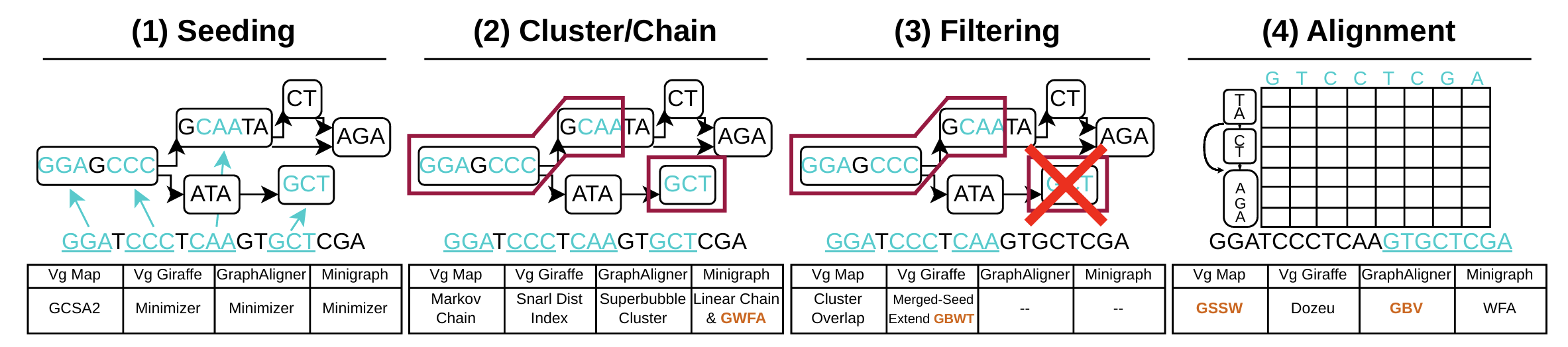Fig. 1: Sequence To Graph Mapping Pipeline.

Extending the steps used in linear mapping to work with a graph reference introduces new design trade-offs, increases complexity, adds dependencies, and causes control divergence. For instance, most Seq2Graph tools use minimizer-based seeding, which is faster than the FM Index-based seeding used in some linear Seq2Seq mapping [16]. Linear clustering and chaining techniques typically rely on distance calculations between seeds, computed as the difference between coordinate locations on the reference. In graph mapping, however, this distance corresponds to the shortest path length, which is complicated by the presence of cycles and requires graph traversal or memoization in large data structures. Additionally, graph references introduce new dependencies in alignment, as discussed in Section III. These complexities mean that Seq2Graph algorithms can take hours for a single individual and are often run iteratively or across multiple samples.

Figure 2 shows a breakdown of time spent in four different mapping tools categorized into seeding, clustering/chaining, filtering, and alignment steps. GraphAligner and Minigraph are evaluated for long reads and long assemblies. While Vg Map and Vg Giraffe are characterized for short reads. We discuss a few observations below.

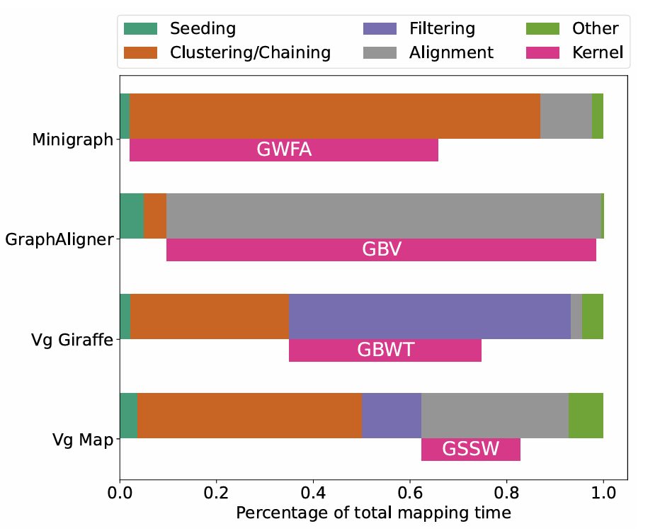
Fig. 2: Seq2Graph Timing Breakdown: Function level timing breakdown extracted with VTune. The tools are designed for and evaluated on different datasets covering short reads, long reads, and assemblies (see Sec IV-B).

In contrast to linear mapping where seeding can take $38\%$ of the runtime [1], we find that Seq2Graph tools spend at most $5\%$ of the runtime in this step. This is partly because minimizer seeding is more popular in Seq2Graph than Seq2Seq, and minimizer trades seeding accuracy for shorter runtime. Second, even for Vg Map, which uses a modified graph based FMIndex [17], the complexity of the subsequent stages dominates.

In the clustering/chaining and filtering steps, some tools employ advanced heuristics to minimize the computational burden on downstream alignment. Minigraph, designed for long sequences where alignment is particularly slow, thus uses 2D dynamic programming within the chaining stage to reduce number of downstream alignments. From this stage, we extract the Graph Wavefront Alignment (GWFA) kernel, which accounts for $75\%$ of the total clustering and chaining time. Although used during chaining, GWFA closely mirrors the computational pattern of dynamic programming used in alignment [1].

Vg Giraffe also features a sophisticated and time-consuming filtering step, which performs light-weight seed extension through the graph using operations on the Graph Burrows-Wheeler Transform Index. The pink bar in Figure 2 illustrates the time spent on all GBWT index operations. For our benchmark suite, we select a single representative operation as the GBWT kernel.

In contrast, GraphAligner uses lightweight clustering ($5\%$ of runtime), and spends the remaining $90\%$ on alignment. To make this feasible for long reads, GraphAligner uses aggressive heuristics (non affine-gap scoring) in the alignment step which trade accuracy to make performance manageable. We extract the the graph bitvector kernel, GBV from the alignment stage of GraphAligner for our benchmark suite.

Vg Map falls between these extremes, with significant time distributed across all stages. From the alignment stage, we extract the Graph SIMD Smith-Waterman (GSSW) kernel, as it is dominated by a single hot function. In contrast, the clustering and chaining stages are fragmented across numerous shorter function calls.

In summary, the mapping tools we analyzed make distinct trade-offs between accuracy and performance across various stages. While we might expect similar tools to allocate comparable proportions of time to each stage, we instead observe that different tools prioritize different stages. No single step or computational pattern stands out as a clear bottleneck, suggesting that all stages could benefit from optimization and acceleration.

B. Graph Building

There are two popular graph-building pipelines in panegenomics research. Both are commonly used and have different merits. Where Minigraph-Cactus's (MC) [14] run time scales with the number of input genomes, the PanGenome Graph Builder (PGGB) [15] prioritizes eliminating reference bias. Both pipelines begin with a collection of sequences and construct a graph in four computational stages (see Figure 3): (1) Alignment identifies matching sub-sequences within the input reference sequences; (2) Graph induction constructs a pangenome graph from the matches; (3) Polishing refines the pangenome graph, for instance, by filtering out short variations; (4) Visualization constructs a 2D representation of the graph for evaluation. These four steps are part of an interactive, iterative, and time-consuming process where scientists build the graph, evaluate its 2D representation, manually update the graph-building parameters, and repeat. For real-world pangenome graphs, each iteration requires hours to complete [18]. Performance improvements would enable researchers to evaluate a greater parameter space, resulting in higher-quality pangenome graphs.

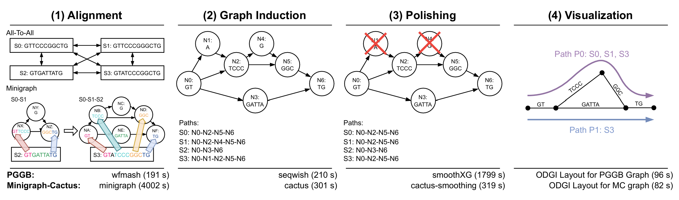Fig. 3: Pangenome Graph Building Pipeline: Run time was measured for both pipelines for processing a small pangenome consisting of 14 high-quality, whole-chromosome chromosome 20 assemblies (see Sec. IV-B).

The alignment stage differs significantly between the two pipelines. Minigraph-Cactus (MC) iteratively grows a pangenome starting from a single reference using Minigraph Seq2Graph mapping, as illustrated in Figure 3.1. The choice of this starting sequence affects the final quality, resulting in potential reference bias. In contrast, PGGB removes reference bias by computing pairwise alignments for all combinations of input sequences. The all-to-all alignments are generated using wfmash [19], which combines the WaveFront Algorithm (WFA) [20] with MashMap [21]. Although all-to-all alignment scales quadratically with the number of sequences, wfmash can be faster than MC for few inputs, depending on the configuration, such as identity threshold and alignment block size. Wfmash is dominated by linear WFA alignment, which has been included in benchmarks before [8].

The graph induction stage constructs an (initial) pangenome graph using the previously created alignments. Cactus, from the MC pipeline, converts the previously generated minigraph alignments into a cactus graph. Here, performance is constrained by the Adaptive Banded Partial Order Alignment algorithm (abPOA) [22], a variation of which is found in previous benchmark suites [1]. Seqwish [23], the tool used by PGGB, utilizes wfmash's all-to-all alignments and performs a translocase step on them, mapping matching nucleotides to pangenome graph nodes. Subsequently, seqwish compresses multiple non-branching nodes into a single node and inserts the corresponding paths through the graph. We extract the translocase step as the TC kernel, as it accounts for more than $75\%$ of the compute time.

The initial pangenome graphs contain complex local structures, which can lead to issues in downstream analysis. These undesired structures are removed in the polishing step. For instance, MC uses gaffix [24] and other algorithms to remove redundant paths and complex structures, such as poorly aligned regions. However, we did not identify a bottleneck in MC smoothing. SmoothXG [25], from the PGGB pipeline, similarly removes small cyclic regions within the graph. Its compute time is dominated by Partial Order Alignment (POA), which takes about $80\%$ of its run time. POA, a dynamic programming kernel, is part of prior benchmarks [1] and has been a target of hardware acceleration [26].

As modern pangenome graphs are large and complex datasets, researchers require tools for exploring their inherent structure. Visualizations are one such tool. ODGI [27], a software toolkit for exploring pangenome graphs, includes a subcommand to generate layouts for 2D visualizations of pangenome graphs in both pipelines. It employs the iterative Path-Guided Stochastic Gradient Descent (PGSGD) [18], [28] algorithm to compute the layout by defining it as an optimization problem. As PGSGD dominates the run time of this task, we extract it as the PGSGD kernel.

III. PANGENOMICS BENCHMARK SUITE

We extract hot snippets of code from our six tools and release them as a benchmark suite. We discuss these kernels in depth here.

Graph SIMD Smith-Waterman (GSSW): Graph SIMD Smith-Waterman [29] is a dynamic programming algorithm used in Vg Map to map read fragments ($\approx 100$ base pairs) to acyclic subgraphs extracted around seed hit locations from the pangenome reference graph.

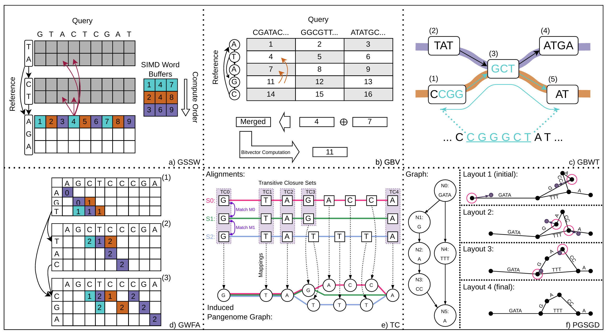
It is based on linear Smith-Waterman [30], which fills in an $n\times m$ dynamic programming (DP) matrix where $m$ is the length of the query, and $n$ is the length of a reference substring. The computation of cell $(i,j)$ is dependent on the maximum of cells $(i,j - 1)$, $(i - 1,j - 1)$ and $(i - 1,j)$, causing Smith-Waterman to process these cells serially. Farrar's algorithm breaks the dependency on the $(i,j - 1)$ cell by speculating the score in cell $(i,j - 1)$ is not the maximum of the three dependencies, and recomputing when it mispeculates. This lets Farrar's strip mine across a row to get SIMD parallelism [31]. This is illustrated in Figure 4 a) for a word size of three, where cells of the same color are packed into a SIMD（Single Instruction, Multiple Data）word.

GSSW uses SIMD Smith-Waterman, but instead of a linear reference on the i-axis, it aligns to a topological sort of a subgraph of the reference with directed edges between nodes, Figure 4 a). Cells within the body of a node are computed with SIMD Smith-Waterman, but cells in the first row of a node depend on the max of all parents, as shown in figure 4 a) with red arrows. This node initialization is done separately, causing the algorithm to alternate between dense SIMD regions and indirect graph accesses.

Many alignment algorithms will employ sophisticated pruning heuristics to compute fewer cells in the DP matrix, but this can make the algorithms harder to parallelize, and sometimes less accurate. GSSW computes more cells than are necessary, which keeps the algorithm simple, and vectorizable. It is slower, but highly accurate, and a good target for hardware acceleration.

Fig.4:KernelExplanatoryFigures.

Graph Myers's Bitvector (GBV): Graph Myers's Bitvector [32] is a dynamic programming algorithm used to align long reads in GraphAligner. As shown in Figure 2, GraphAligner exerts little effort filtering seed hits, which results in many alignments. This, and the presence of long reads create abundant work for the alignment stage. GBV manages this by trading alignment quality for computational efficiency.

Myers's bitvector [33], does not support the sophisticated affine gap scoring method used in Smith-Waterman. This breaks the dependency on the $(i,j - 1)$ cell discussed in GSSW, and allows Myers to store rows as bitvectors. Rows are operated on in parallel with SIMD width equal to the word size of the machine, 64 by default.

In Graph Myers's bitvector, each row represents a one-base pair node with directed edges to its children, Figure 4 b). This makes each row dependent on its parent rows (i.e. nodes), shown with red arrows in Figure 4 b). To compute the next row, all the parents are merged into one bitvector, and then that bitvector is used to compute the row.

Since GBV aligns to cyclic graphs, the current row being computed, $R_{i}$, may change the value of its parent $R_{p}$. Thus, some rows will need to be recomputed until the solution stabilizes. To keep track of the nodes that need to be recomputed, GBV pushes rows to a priority queue when their parent changes, and processes them in the queue order.

These changes to the algorithm made to accommodate graphs introduce unpredictable branching behavior to GBV, but the high level of SIMD parallelism makes the algorithm a fast alternative to more accurate affine scoring methods.

---

Graph Burrows-Wheeler Transform (GBWT): Vg Giraffe uses the GBWT Index [34] in the filtering step of the mapping pipeline, Figure 1.3, to extend clustered seed hits. The seed hit is extended within a node via exact matches tolerating up to four mismatches. When the seed hit extension reaches the end of a node, it calls a GBWT Index function to find the next possible nodes it can continue into. Many paths lead to unrealistic results, so we only follow paths where a known haplotype exists. For example, in Figure 4 c) there is a haplotype $1 \rightarrow 3 \rightarrow 5$, and another haplotype $2 \rightarrow 3 \rightarrow 4$, but since the seed extension has already gone through $1 \rightarrow 3$, it cannot go to 4 because there is no haplotype.

More generally, this is accomplished with a GBWT Index function, find that takes a sequence of nodes, $S = (s_1, s_2, \ldots, s_n)$ as input and returns all possible next nodes. This function is representative of operations using GBWT Index, and so we extract it as a kernel, even though Vg Giraffe actually makes use of many GBWT Index functions.

The GBWT Index is a haplotype-aware graph FM-Index [35] that uses last-first mapping to look up nodes. It is built on a multi-string Burrows-Wheeler Transform (BWT) applied to haplotype paths through the graph. Unlike the linear FM-Index, which applies the BWT to a single string composed of base pairs, the GBWT Index is based on multiple sequences (haplotype paths) of node IDs in the graph, which enables graph specific optimizations to the index.

---

Graph Wavefront Algorithm (GWFA): The Graph Wavefront Algorithm [36] is used in Minigraph to bridge gaps between seed hits (also called anchors) in different nodes. Although it is used in the chaining step, it uses dynamic programming and is computationally more similar to GSSW and GBV. Given two anchors, it finds a path (sequence of nodes) connecting them. This requires less accuracy than base-level alignment, so GWFA uses non-affine gap scoring.

Linear WFA [20] computes cells along diagonals in the matrix. At each iteration, it computes wavefront $W_d$, the set of furthest reaching (most down and right) cells along each diagonal with edit distance less than or equal to $d$. For example, in dynamic programming matrix (2) of Figure 4 d), $W_2$ is the set containing, the blue cell, the orange cell, and the lower right purple cell, all marked with a score of 2. It computes the wavefront by extending each diagonal until the next edit. Some diagonals will go further than others resulting in control divergence, and irregular accesses.

In the graph version depicted in Figure 4 d), each node has its own dynamic programming matrix with the query on one axis, and the node on the other axis. The matrices are connected by edges corresponding to the edges between nodes. When a diagonal reaches the end of a node, it expands the wavefront to include a continuation in each of its children, as shown by the blue diagonal in Figure 4 d). This leads to a larger wavefront with cells scattered across different nodes resulting in irregular accesses.

Despite this, GWFA is the fastest alignment algorithm reviewed [36] because it computes much fewer cells of the DP-Matrix than the others.

---

Transclosure (TC): PGGB [15] utilizes Seqwish [23] to induce pangenome graphs from input sequences and their respective all-to-all alignments. Seqwish’s run time is dominated by its transclosure (TC) kernel, which generates the set of pangenome graph nodes: each pairwise alignment from the all-to-all alignments specifies matching characters in their sequences. For instance, the match M0 between sequences S0 and S1 in Figure 4 e) creates the Transitive Closure set TC0. These sets are extended via the transitive property. For example, M1 matches S1 to S2, so S2’s character is added to TC0. To generate all closures, TC iterates over the set of input characters and locates their matches, as well as matches connected via the transitive property. Connected matches are found efficiently using a binary search, as the matches are sorted by their sequences in a prior step. Each transitive closure is then mapped to a graph node.

TC introduces a critical new task in the domain of pangenome graph-building. Unlike many other workloads in genomics, TC does not use alignment. Instead, it leverages clever data structures, such as implicit interval trees [37], which are used for efficient union-find operations but require high-performance sorting steps [38] for efficient data access. For real-world pangenome graphs, these data structures require 100s of GBs of memory space. To enable memory-limited systems to perform the TC computation, TC memory-maps these structures to files. Thus, TC is constructed from a set of heterogeneous algorithms, including sorting and union-find.

---

Path-Guided Stochastic Gradient Descent (PGSGD): ODGI [27] employs Path-Guided Stochastic Gradient Descent (PGSGD) [18], [28] to generate 2D layouts of pangenome graphs. Visualization is used iteratively in the graph-building pipeline to assess the quality of the graph and is computationally intensive, taking hours to generate for real-world chromosome-scale pangenomes [18]. PGSGD takes a pangenome graph as input and generates a layout file containing 2D coordinates for each pangenome graph node.

PGSGD iteratively optimizes the layout to match the distances between nodes in the pangenome graph. Figure 4 f demonstrates this. In the initial Layout 1, the line lengths poorly match the corresponding sequence lengths. Furthermore, the structure of the pangenome is difficult to grasp due to a twist in its complex region. In each update step, two anchors within the layout are randomly selected, and their coordinates are adjusted to better match the corresponding path-distance in the pangenome graph (Figure 4 e, left). In Layout 1, the left anchor of NO and the anchor between N1 and N2 are chosen. Since they are too far apart, PGSGD moves them closer together. This results in Layout 2, where two anchors are pushed away from each other as they are too close. After numerous update steps, the distances within the layout converge to their corresponding path-distances, as shown by Layout 4. As PGSGD contains millions of update steps, they are parallelized across threads using the lock-free Hogwild! approach [39]. In the rare case that a race condition occurs, future iterations will quickly correct the incorrect update.

PGSGD introduces an entirely new task to the pangenomics workflow utilizing the stochastic gradient descent optimization. It also requires pseudo-random memory accesses to the graph and uses the Hogwild! parallelization method, which distinguishes it from other workloads.

IV. METHODOLOGY

A. Procedure and Tools

We first perform VTune [40] hotspot analysis and manual timing instrumentation on realistic datasets for end-to-end workflows at the tool level to identify hotspots. We then isolate kernels from the hotspots for our benchmark suite. The inputs for each kernel is generated by running the original tool on the full dataset and recording the kernel function arguments during execution. To make the benchmark suite accessible for a typical server, we subsample most datasets down to a couple of Gigabytes, and around 20s of kernel runtime. This does not significantly change results, except in the case of GBWT where the index size affects caching. For GBWT we use the full graph GBWT Index.

We then perform three analyses for each kernel using VTune: microarchitecture exploration to understand hardware utilization, cache miss rates to find misses per kilo instruction, and a customized version of MICA PIN [41] [42] to get a dynamic instruction count. The scripts for running these analyses, benchmarks, and datasets are all open-sourced on our github. Lastly, we perform three case studies on selected kernels, described in section VI.

B. Datasets

TABLE I: Dataset Information for Kernels

Kernel	Dataset
GSSW	MC Graph; HG002 Illumina Short Reads
GBWT	MC Graph GBWT Index; Randomly Sampled Queries
GBV	MC Graph; Hg002 PacBio 15kb/20kb Long Reads
GWFA	MC Graph; T2T Hg002 Assembly Contig
TC	14 Contigs From HPRC & T2T; Yeast
PGSGD	14 Contigs From HPRC & T2T; DRB1-3123

The datasets we use are shown in table I. Except in the case of GBWT, which uses the full genome, all human data is from chromosome 20. This makes problems tractable for benchmarking with less than 125GB of memory footprint.

Seq2Graph mapping: We use the Minigraph-Cactus (MC) constructed graph from HPRC [5] [43] as a reference. We generate GBWT inputs by randomly sampling subsequences from the haplotypes in the graph with lengths between 1 and 100. We use Illumina HiSeq short reads (150bp), and PacBio HiFi long reads (15000bp and 20000bp), both from sample HG002 of the HPRC. To isolate the chromosome 20 reads, we first align all reads to the T2T HG002 reference [44] using Minimap2 for long reads, and BWA-Mem2 for short reads. We then filter out reads that did not align to chromosome 20.

Graph Building: We take 14 high-quality chromosome 20 assemblies, including T2T CHM13 [44] and 13 from HPRC [45]. For TC and PGSGD, human data is too slow for PIN analysis, so we use Yeast [46] and DRB1-3123 [47] datasets for PIN analysis only.

C. Machine Configuration

TABLE II: System Configuration.

Component	Details
CPU	Intel Xeon Gold 6326 2.90 GHz; 16 cores/32 threads per socket; 2 sockets
L1 I cache	48Kb, 8-way
L1 D cache	32Kb, 12-way
L2 cache	1.25Mb, 20-way
L3 cache	48Mb (Shared), 12-way
Memory	8 × 16GB DDR4 3200MHz

We evaluate kernels and do microarchitectural analyses using the server in table II. We evaluate tools on full datasets using a dual-socket Intel Xeon CPU E5-2697 v3, with up to 500GB RAM as needed.

V. MICROARCHITECTURAL ANALYSIS

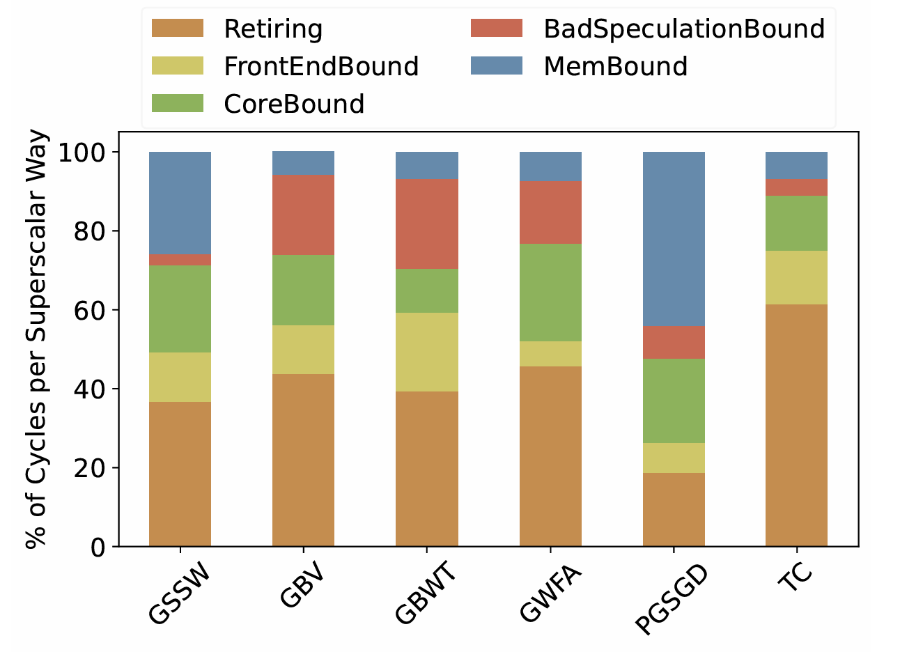
Fig. 5: Top-Down Microarchitectural Analysis for Our Benchmarks: The y-axis shows the fraction of superscalar ways retiring or stalled for different reasons.

TABLE III: Kernel IPC (4-way CPU core)

Kernel	GSSW	GBV	GBWT	GWFA	PGSGD	TC
IPC	1.77	2.23	1.94	2.32	1.14	3.14

In this section we analyze the microarchitectural bottlenecks of the extracted benchmarks. Figure 5 shows a breakdown of bottlenecks collected from top-down VTune microarchitecture analysis [48]. The y-axis shows the fraction of superscalar ways per cycle that are doing useful work (Retiring) or stalled for some other reason. If an instruction is issued but never retires, that superscalar way is classified as Bad Speculation. In our benchmarks, this is mostly attributed to branch misprediction. If an instruction was not issued because the backend of the pipeline was stalled, we classify the way as CoreBound or MemoryBound. If the backend had free slots, but there was no micro-op to dispatch, the way is classified as FrontEndBound. Table III shows the IPC for each kernel.

The results show that dynamic programming kernels GSSW, GBV, and GWFA, are core bound. This is understandable because these are compute-intensive kernels with complex data dependencies on previous cells, but unlike GBV and GWFA, GSSW uses affine gap scoring, which triples the memory footprint. Because of this, and other memory bottlenecks discussed in Section VI-A, GSSW is also memory bound.

In contrast, GBV is limited by branch misprediction attributed partly to the traceback step implemented within the kernel and partly to the merge operations between parent cells (Figure 4 b)). The merge operation is distinctly a graph-based step, where data from incoming edges is combined.

GWFA is similarly bound by bad speculation. We trace the source of the branch misprediction to two regions of the code. The first performs extension along the diagonal until a mismatch. This code has poor branch behavior due to data-dependent control flow. The second hotspot is part of the graph algorithm that checks if a diagonal has reached the end of a node. Although the linear WFA algorithm must also check the boundary, this has a more predictable branch behavior than the graph counterpart.

Prior work has found linear BWT-based FM-Index to be memory bandwidth-intensive [1], [49], but GBWT is not memory bound. Due to the limited alphabet of four base pairs, substrings of the reference text are often repeated, so for a short substring there are many possible prefixes, any of which could be the next hop. This results in unpredictable memory accesses to the compressed occurrence table [35]. In contrast, GBWT is a multistring BWT over haplotypes (sequences of node IDs). These haplotypes are less likely to repeat themselves, so for a given substring, there are usually only a handful of prefixes. This limits the range of lookups, making index search queries more likely to access nearby nodes and therefore adjacent entries in the occurrence table [34]. The lack of memory bottlenecks exposes branch misses and frontend stalls from the data dependent control flow in GBWT.

Unlike the alignment kernels which align reads to small localized subgraphs, graph visualization is performed on the entire graph, resulting in a much larger memory footprint (1.7Gb for chromosome 20). To ensure the generation of high-quality layouts, PGSGD performs uniform random queries to this structure, independent of the graph structure. This results in a memory bottleneck. Furthermore, the coordinate update involves multiple divisions and square-root operations (e.g., for computing the Pythagorean theorem). Memory and core-boundness result in a low IPC.

TC also operates on a full chromosome dataset composed of multiple linear alignments, but it's accesses are much more regular. TC performance is dominated by efficient accesses to optimized data structures (like implicit interval trees [37] and atomic bitvectors [50]), the simple appending of data to files, and highly optimized sorting [38], resulting in a high IPC.

Perhaps surprisingly, we do not observe memory bottlenecks from indirect graph accesses in the kernels we have reviewed. GSSW, GBV, and GWFA operate on subgraphs which fit in the cache. GBWT exhibits good locality because of its graph representation and cache-friendly optimizations. PGSGD is memory bound because of its random sampling method, not because of the graph structure, and TC utilizes efficient data structures and can exploit some spatial locality, e.g., during the bitvector accesses.

Figure 6 shows cache misses per kilo-instructions. We note that the dynamic programming kernels rarely miss the $\boldsymbol{l3}$ indicating that they are not making many irregular accesses to the full pangenome. Instead, they mostly miss the $\boldsymbol{l1}$. This is likely because they perform local alignment on small subgraphs. In contrast, PGSGD stands out with a high miss rate across all levels of the cache. This is because PGSGD has completely random accesses to the graph, that does not fit in any level of the cache, despite using a cache-optimized data layout [18].

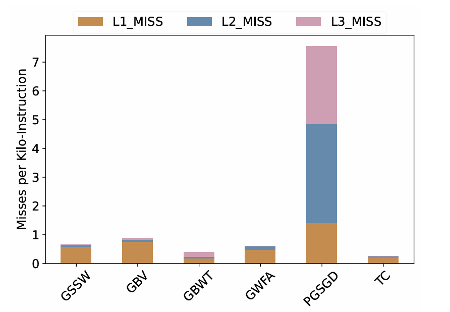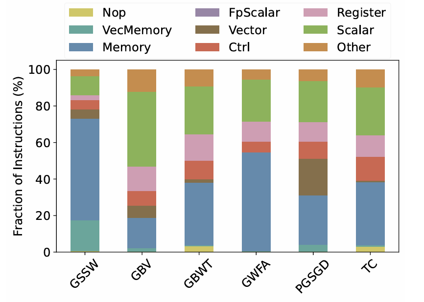Fig. 6: Misses per Kilo-Instruction for Our Benchmarks: collected with VTune: These counts are exclusive, that is if an instruction misses in $l2$ it is not shown as an $l1$ miss.	Fig. 7: Dynamic Instruction Count for Our Benchmarks: collected with Intel PIN.

Figure 7 gives a dynamic instruction count for each of the kernels. Because x86 is a CISC instruction set, many instructions fit multiple categories, for instance an instruction might be a vector control flow operation. We chose to bin instructions hierarchically in the order they appear in the legend (read top to bottom, left to right). We classify mov instructions between registers as Register instructions.

We analyze usage of vector instructions in the dynamic programming benchmarks: GSSW, GBV, GWFA. Notice that GWFA has fewest vector instructions. This is surprising because previous work suggests that linear WFA is easily autovectorized [20]. Our results indicate that graph related modifications prevent the compiler ($\mathrm{g + + 11}$) from autovectorizing the code. Manually vectorizing the code could result in performance gains for GWFA. In contrast, we see GSSW has a significant fraction of vector and memory operations because it is a memory-bound, hand-vectorized code. GBV bitvectors are restricted to 64 bits in the code, so these operations are classified as scalar. We also observe that PGSGD makes heavy use of SSE instructions, which are classified as vector, but a closer look reveals that these are mostly SSE floating point scalar operations (e.g. MULSD) used in distance calculations. The other kernels, GBWT and TC, consist mostly of scalar operations. GBWT alternates between scalar operations on compressed data and lookups to find the next node, resulting in a mix of scalar and memory operations.

Fig. 8: Comparison of Linear and Graph Mapping: Microarchitectural analysis of Graph SIMD Smith-Waterman (GSSW) and linear Striped Smith-Waterman (SSW) collected with Intel VTune.

VI. CASE STUDIES

A. Seq2Seq and Seq2Graph Comparison

In this case study, we compare GSSW with linear Stripped Smith-Waterman (SSW). GSSW is a direct extension of the SSW codebase; both libraries are implemented in C by the same authors and utilize Farrar's method of parallelization. We generate inputs for SSW by running BWA-MEM [16] on short reads from chromosome 20 and using HG002 assembly as reference (Section IV). The input traces to the alignment function are recorded and subsequently used for SSW. For GSSW, we align the same set of input reads to the Minigraph-Cactus graph using Vg Map.

Figure 8 shows microarchitectural analysis of the two kernels. We find the proportions are almost identical, except GSSW has $\approx 3\times$ more memory stalls. We trace the source of these stalls to three lines in the source code that write the SIMD buffers used for score computation back to the Dynamic Programming (DP) matrix. The buffers contain packed striped data, as shown in Figure 4 a). The writeback needs to unpack them into the array and exhibits poor locality.

In linear alignment, the computation of a row $i$ depends only on row $i - 1$. Therefore, SSW stores only the previous row. In contrast, graph alignment algorithm GSSW stores all rows of the dynamic programming matrix, as row $i$ may access any nodes it depends on (see incoming edges in Figure 4 a). However, we observe that within a node, the rows exhibit linear dependencies, meaning these rows do not need to be stored. This optimization could improve performance by avoiding the costly writebacks from SIMD buffers to DP matrix.

B. Graph Variation

Compared to linear references, graphs are much more diverse. Two linear references generally exhibit the same computational behavior, but two graphs can represent the same pangenome with wildly different runtimes. We explore these differences in two case studies:

In our first experiment, we compare two graphs of Chromosome 20 constructed from HPRC [5] assemblies using the Minigraph-Cactus and PGBG pipelines, respectively referred to as M-Graph and P-Graph. Both graphs are widely used and offer different merits. We align an assembly derived from CHM13hTERT human cell line [51] with the Minigraph mapping tool and record the input traces to GWFA for analysis. Figure 9 shows the microarchitecture analysis, and total clock cycles GWFA ran for each graph. Although the microarchitectural utilization is similar, we observe that the P-Graph achieves a $56\%$ shorter runtime. Recall that GWFA is employed in the clustering/chaining step to identify paths between anchors. Our analysis shows that the average gap size between anchors is $96$ bp for the M-Graph and $86$ bp for the P-Graph. The larger gaps in the M-Graph likely increases chaining complexity, contributing to its longer runtime.

In our second experiment, we split each node in the MGraph with more than $8$ base pairs into a chain of nodes with $8$ base pairs each to create the Split-M-Graph. This brings the average node length from $27.22$ base pairs in the M-Graph to $6.89$ base pairs in the Split-M-Graph. We generate inputs for the GSSW kernel using Vg Map.

As shown in Figure 10, the Split-M-Graph achieves a shorter runtime than the full M-Graph, despite similar microarchitectural utilization. Analyzing the inputs generated by Vg Map for GSSW, we observe that the average size of the reference subgraphs used as kernel inputs decreases from $450$ base pairs in the M-Graph to $233$ base pairs in the Split-M-Graph. This reduction explains the faster runtime. The Split-M-Graph introduces finer-grained nodes, enabling the chaining, clustering, and filtering steps to more precisely identify reference graph regions, thereby generating smaller subgraphs for alignment.

Both these experiments confirm that the graph input has a large effect on the runtime of mapping algorithms and they indicate that the difference in this runtime is heavily dependent on the quality of the seeding/clustering/chaining/filtering algorithms before alignment.

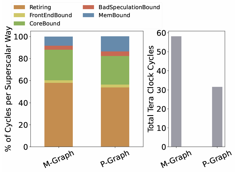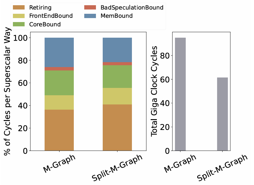Fig. 9: Comparison of M and P Graph with GWFA: GWFA runs on Minigraph-Cactus and Pggb graphs. Left: microarchitectural analysis. Right: number of cycles GWFA took to finish.	Fig. 10: Comparison of M and Split-M Graph with GSSW: GSSW runs on Minigraph-Cactus graph and modified Minigraph-Cactus graph with split nodes. Left: microarchitectural analysis. Right: number of cycles GSSW took to finish.

VII. BACKGROUND AND RELATED WORK

BioPerf and BioBench are some of the earliest genomics benchmarks [6], [7]. These include a diverse set of kernels for DNA and Protein analysis including alignment and phylogenetic analysis. GenomicsBench profiles more recent tools from de novo assembly, reference-based assembly, and metagenomics on CPU and GPU [1]. GenArchBench ports the kernels from GenomicsBench to ARM for HPC, and it adds some new kernels, notably WFA and Myers's Bitvector Alignment [8]. Genomics-GPU is another benchmark suite written specifically for GPU containing many kernels from the mapping pipeline [9]. PangenomicsBench stands apart from these as the first benchmark suite targeting pangenomics, which we have shown to be an interesting subfield with different computational characteristics.

VIII. CONCLUSION

In this work, we examined two pangenomic workflows and analyzed widely used tools for these workflows. From this analysis, we identified six key computational kernels and developed a new benchmark suite, PangenomicsBench. We characterized these kernels based on their microarchitectural bottlenecks and conducted two case studies to explore the effects of input graph variation and the differences between linear and graph alignment. Our findings reveal the following: (a) Contrary to expectation, graph-based applications are not constrained by memory access to the graph as they operate on smaller subgraphs. (b) The complexity of graph structures necessitates algorithms with higher control flow complexity, which impacts performance. (c) Pangenomic mapping algorithms are highly sensitive to the structure of the reference graph. (d) Pangenomic graph construction introduces fundamentally different algorithms compared to those used in linear genomics workflows. (e) There are opportunities for software optimizations in existing code.

[1] A. Subramaniyan, Y. Gu, T. Dunn, S. Paul, M. Vasimuddin, S. Misra, D. Blaauw, S. Narayanasamy, and R. Das, "Genomicsbench: A benchmark suite for genomics," in 2021 IEEE International Symposium on Performance Analysis of Systems and Software (ISPASS). IEEE, 2021, pp. 1-12. [2] A. Guarracino, S. Buonaiuto, L. G. de Lima, T. Potapova, A. Rhie, S. Koren, B. Rubinstein, C. Fischer, J. L. Gerton et al., "Recombination between heterologous human acrocentric chromosomes," Nature, vol. 617, no. 7960, pp. 335-343, 2023. [3] "Computational pan-genomics: status, promises and challenges," Briefings in bioinformatics, vol. 19, no. 1, pp. 118-135, 2018. [4] R. M. Sherman and S. L. Salzberg, "Pan-genomics in the human genome era," Nature Reviews Genetics, vol. 21, no. 4, pp. 243-254, 2020. [5] W.-W. Liao, M. Asri, J. Ebler, D. Doerr, M. Haukness, G. Hickey, S. Lu, J. K. Lucas, J. Monlong, H. J. Abel et al., "A draft human pangenome reference," Nature, vol. 617, no. 7960, pp. 312-324, 2023. [6] D. A. Bader, Y. Li, T. Li, and V. Sachdeva, "Bioperf: A benchmark suite to evaluate high-performance computer architecture on bioinformatics applications," in IEEE International, 2005 Proceedings of the IEEE Workload Characterization Symposium, 2005. IEEE, 2005, pp. 163-173. [7] K. Alhayarkaroglu, A. Jaleel, X. Wu, M. Franklin, B. Jacob, C.-W. Tseng, and D. Yeung, "Biobench: A benchmark suite of bioinformatics applications," in IEEE International Symposium on Performance Analysis of Systems and Software, 2005. ISPASS, 2005. IEEE, 2005, pp. 2-9. [8] L. López-Villellas, R. Langarita-Benítez, A. Badouh, V. Soria-Pardos, Q. Aguado-Puig, G. López-Paradís, M. Doblas, J. Setoain, C. Kim, M. Ono et al., "Genarchbench: A genomics benchmark suite for arm hpc processors," Future Generation Computer Systems, vol. 157, pp. 313-329, 2024. [9] Z. Liu, S. Zhang, J. Garrigus, and H. Zhao, "Genomics-gpu: A benchmark suite for gpu-accelerated genome analysis," in 2023 IEEE International Symposium on Performance Analysis of Systems and Software (ISPASS). IEEE, 2023, pp. 178-188. [10] M. Rautiainen and T. Marschall, "Graphaligner: rapid and versatile sequence-to-graph alignment," Genome biology, vol. 21, no. 1, p. 253, 2020. [11] E. Garrison, J. Sirén, A. M. Novak, G. Hickey, J. M. Eizenga, E. T. Dawson, W. Jones, S. Garg, C. Markello, M. F. Lin et al., "Variation graph toolkit improves read mapping by representing genetic variation in the reference," Nature biotechnology, vol. 36, no. 9, pp. 875-879, 2018. [12] J. Sirén, J. Monlong, X. Chang, A. M. Novak, J. M. Eizenga, C. Markello, J. A. Sibbesen, G. Hickey, P.-C. Chang, A. Carroll et al., "Pangenomics enables genotyping of known structural variants in 5202 diverse genomes," Science, vol. 374, no. 6574, p. abg8871, 2021. [13] H. Li, X. Feng, and C. Chu, "The design and construction of reference pangenome graphs with minigraph," Genome biology, vol. 21, pp. 1-19, 2020. [14] G. Hickey, J. Monlong, J. Ebler, A. M. Novak, J. M. Eizenga, Y. Gao, T. Marschall, H. Li, and B. Paten, "Pangenome graph construction from genome alignments with minigraph-cactus," Nature biotechnology, pp. 1-11, 2023. [15] E. Garrison, A. Guarracino, S. Heumos, F. Villani, Z. Bao, L. Tattini, J. Hagmann, S. Vorbrugg, S. Marco-Sola, C. Kubica et al., "Building pangenome graphs," Nature Methods, pp. 1-5, 2024. [16] H. Li, "Aligning sequence reads, clone sequences and assembly contigs with bwa-mem," arXiv preprint arXiv:1303.3997, 2013. [17] J. Sirén, "Indexing variation graphs," in 2017 Proceedings of the nineteenth workshop on algorithm engineering and experiments (ALENEX). SIAM, 2017, pp. 13-27. [18] J. Li, J.-N. Schmelzle, Y. Du, S. Heumos, A. Guarracino, G. Guidi, P. Prins, E. Garrison, and Z. Zhang, "Rapid gpu-based pangenome graph layout," in Proceedings of the International Conference for High Performance Computing, Networking, Storage, and Analysis, ser. SC '24. IEEE Press, 2024. [Online]. Available: https://doi.org/10.1109/SC41406.2024.00035 [19] A. Guarracino, N. Mwaniiki, S. Marco-Sola, and E. Garrison, "wfmash: whole-chromosome pairwise alignment using the hierarchical wavefront algorithm. GitHub," 2021. [Online]. Available: https://github.com/waveygang/wfmash

[1] A. Subramaniyan, Y. Gu, T. Dunn, S. Paul, M. Vasimuddin, S. Misra, D. Blaauw, S. Narayanasamy, and R. Das, "Genomicsbench: A benchmark suite for genomics," in 2021 IEEE International Symposium on Performance Analysis of Systems and Software (ISPASS). IEEE, 2021, pp. 1-12. [2] A. Guarracino, S. Buonaiuto, L. G. de Lima, T. Potapova, A. Rhie, S. Koren, B. Rubinstein, C. Fischer, J. L. Gerton et al., "Recombination between heterologous human acrocentric chromosomes," Nature, vol. 617, no. 7960, pp. 335-343, 2023. [3] "Computational pan-genomics: status, promises and challenges," Briefings in bioinformatics, vol. 19, no. 1, pp. 118-135, 2018. [4] R. M. Sherman and S. L. Salzberg, "Pan-genomics in the human genome era," Nature Reviews Genetics, vol. 21, no. 4, pp. 243-254, 2020. [5] W.-W. Liao, M. Asri, J. Ebler, D. Doerr, M. Haukness, G. Hickey, S. Lu, J. K. Lucas, J. Monlong, H. J. Abel et al., "A draft human pangenome reference," Nature, vol. 617, no. 7960, pp. 312-324, 2023. [6] D. A. Bader, Y. Li, T. Li, and V. Sachdeva, "Bioperf: A benchmark suite to evaluate high-performance computer architecture on bioinformatics applications," in IEEE International, 2005 Proceedings of the IEEE Workload Characterization Symposium, 2005. IEEE, 2005, pp. 163-173. [7] K. Alhayarkaroglu, A. Jaleel, X. Wu, M. Franklin, B. Jacob, C.-W. Tseng, and D. Yeung, "Biobench: A benchmark suite of bioinformatics applications," in IEEE International Symposium on Performance Analysis of Systems and Software (ISPASS). IEEE, 2023, pp. 178-188. [8] L. López-Villellas, R. Langarita-Benítez, A. Badouh, V. Soria-Pardos, Q. Aguado-Puig, G. López-Paradís, M. Doblas, J. Setoain, C. Kim, M. Ono et al., "Genarchbench: A genomics benchmark suite for arm hpc processors," Future Generation Computer Systems, vol. 157, pp. 313-329, 2024. [9] Z. Liu, S. Zhang, J. Garrigus, and H. Zhao, "Genomics-gpu: A benchmark suite for gpu-accelerated genome analysis," in 2023 IEEE International Symposium on Performance Analysis of Systems and Software (ISPASS). IEEE, 2023, pp. 178-188. [10] M. Rautiainen and T. Marschall, "Graphaligner: rapid and versatile sequence-to-graph alignment," Genome biology, vol. 21, no. 1, p. 253, 2020. [11] E. Garrison, J. Sirén, A. M. Novak, G. Hickey, J. M. Eizenga, E. T. Dawson, W. Jones, S. Garg, C. Markello, M. F. Lin et al., "Variation graph toolkit improves read mapping by representing genetic variation in the reference," Nature biotechnology, vol. 36, no. 9, pp. 875-879, 2018. [12] J. Sirén, J. Monlong, X. Chang, A. M. Novak, J. M. Eizenga, C. Markello, J. A. Sibbesen, G. Hickey, P.-C. Chang, A. Carroll et al., "Pangenomics enables genotyping of known structural variants in 5202 diverse genomes," Science, vol. 374, no. 6574, p. abg8871, 2021. [13] H. Li, X. Feng, and C. Chu, "The design and construction of reference pangenome graphs with minigraph," Genome biology, vol. 21, pp. 1-19, 2020. [14] G. Hickey, J. Monlong, J. Ebler, A. M. Novak, J. M. Eizenga, Y. Gao, T. Marschall, H. Li, and B. Paten, "Pangenome graph construction from genome alignments with minigraph-cactus," Nature biotechnology, pp. 1-11, 2023. [15] E. Garrison, A. Guarracino, S. Heumos, F. Villani, Z. Bao, L. Tattini, J. Hagmann, S. Vorbrugg, S. Marco-Sola, C. Kubica et al., "Building pangenome graphs," Nature Methods, pp. 1-5, 2024. [16] H. Li, "Aligning sequence reads, clone sequences and assembly contigs with bwa-mem," arXiv preprint arXiv:1303.3997, 2013. [17] J. Sirén, "Indexing variation graphs," in 2017 Proceedings of the nineteenth workshop on algorithm engineering and experiments (ALENEX). SIAM, 2017, pp. 13-27. [18] J. Li, J.-N. Schmelzle, Y. Du, S. Heumos, A. Guarracino, G. Guidi, P. Prins, E. Garrison, and Z. Zhang, "Rapid gpu-based pangenome graph layout," in Proceedings of the International Conference for High Performance Computing, Networking, Storage, and Analysis, ser. SC '24. IEEE Press, 2024. [Online]. Available: https://doi.org/10.1109/SC41406.2024.00035 [19] A. Guarracino, N. Mwaniiki, S. Marco-Sola, and E. Garrison, "wfmash: whole-chromosome pairwise alignment using the hierarchical wavefront algorithm. GitHub," 2021. [Online]. Available: https://github.com/waveygang/wfmash

[20] S. Marco-Sola, J. C. Moure, M. Moreto, and A. Espinosa, "Fast gap-affine pairwise alignment using the wavefront algorithm," Bioinformatics, vol. 37, no. 4, pp. 456-463, 2021. [21] C. Jain, S. Koren, A. Dilthey, A. M. Philippy, and S. Aluru, "

[43] "Human pangenome reference consortium s3 bucket," accessed: 16-Jun-2024. [Online]. Available: https://s3-us-west-2.amazonaws.com/human-pangenomics/index.html?prefix=pangenomes/freeze/freeze1/minigraph-cactus/hprc-v1.1-mc-grch38/

[44] S. Nurk, S. Koren, A. Rhie, M. Rautiainen, A. V. Bizikadze, A. Mikheenko, M. R. Vollger, N. Altemose, L. Uralsky, A. Gershman, S. Aganezov, S. J. Hoyt, M. Diekhans, G. A. Logsdon, M. Alonge, S. E. Antonarakis, M. Borchers, G. G. Bouffard, S. Y. Brooks, G. V. Caldas, N.-C. Chen, H. Cheng, C.-S. Chin, W. Chow, L. G. de Lima, P. C. Dishuck, R. Durbin, T. Dvorkina, I. T. Fiddes, G. Formenti, R. S. Fulton, A. Fungtamasan, E. Garrison, P. G. S. Grady, T. A. Graves-Lindsay, I. M. Hall, N. F. Hansen, G. A. Hartley, M. Haukness, K. Howe, M. W. Hunkapiller, C. Jain, M. Jain, E. D. Jarvis, P. Kerpedjiev, M. Kirsche, M. Kolmogorov, J. Korlach, M. Kremitzki, H. Li, V. V. Maduro, T. Marschall, A. M. McCartney, J. McDaniel, D. E. Miller, J. C. Mullikin, E. W. Myers, N. D. Olson, B. Paten, P. Peluso, P. A. Pevzner, D. Porubsky, T. Potapova, E. I. Rogaev, J. A. Rosenfeld, S. L. Salzberg, V. A. Schneider, F. J. Sedlazeck, K. Shafin, C. J. Shew, A. Shumate, Y. Sims, A. F. A. Smit, D. C. Soto, I. Sovic, J. M. Storer, A. Streets, B. A. Sullivan, F. Thibaud-Nissen, J. Torrance, J. Wagner, B. P. Walenz, A. Wenger, J. M. D. Wood, C. Xiao, S. M. Yan, A. C. Young, S. Zarate, U. Surti, R. C. McCoy, M. Y. Dennis, I. A. Alexandrov, J. L. Gerton, R. J. O'Neill, W. Timp, J. M. Zook, M. C. Schatz, E. E. Eichler, K. H. Miga, and A. M. Phillippy, "The complete sequence of a human genome," Science, vol. 376, no. 6588, pp. 44-53, 2022. [Online]. Available: https://www.science.org/doi/abs/10.1126/science.abb6987

[45] T. Wang, L. Antonacci-Fulton, K. Howe, H. A. Lawson, J. K. Lucas, A. M. Phillippy, A. B. Popejoy, M. Asri, C. Carson, M. J. Chaisson et al., "The human pangenome project: a global resource to map genomic diversity," Nature, vol. 604, no. 7906, pp. 437-446, 2022.

[46] J.-X. Yue, J. Li, L. Aigrain, J. Hallin, K. Persson, K. Oliver, A. Bergström, P. Coupland, J. Warringer, M. C. Lagomarsino et al., "Contrasting evolutionary genome dynamics between domesticated and wild yeasts," Nature genetics, vol. 49, no. 6, pp. 913-924, 2017.

[47] A. Guarracino, S. Heumos, S. Nahnsen, P. Prins, and E. Garrison, "Optimized Dynamic Genome/Graph Implementation (ODGI)," Sep. 2021. [Online]. Available: https://github.com/pangenome/odgi

[48] A. Yasin, "A top-down method for performance analysis and counters architecture," in 2014 IEEE International Symposium on Performance Analysis of Systems and Software (ISPASS). IEEE, 2014, pp. 35-44.

[49] A. Subramaniyan, J. Wadden, K. Goliya, N. Ozog, X. Wu, S. Narayanasamy, D. Blaauw, and R. Das, "Accelerated seeding for genome sequence alignment with enumerated radix trees," in Proceedings of the 48th Annual International Symposium on Computer Architecture, ser. ISCA '21, 2021.

[50] E. Garrison, "atomicbitvector," 2020. [Online]. Available: https://github.com/ekg/atomicbitvector

[51] "Telomere-to-telomere consortium chm13 project." [Online]. Available: https://github.com/marbi/CHM13