2 GfaViz: Supplementary Information
GfaViz: Flexible and interactive visualization of GFA sequence graphs
PDF: supplementary Data
Gonnella Giorgio, Niklas Niehus and Stefan Kurtz
October 25, 2018
S1 Additional examples of application
S1.1 Alignment graph of long noisy reads
The first step of the assembly of long noisy reads, e.g. obtained by the Pacific Biosciences and Oxford Nanopore sequencing platforms, is usually the computation of local alignment among all read pairs. In GFA 1 only dovetail overlap and containments are supported, but the regions involved in the alignments are often internal. GFA 2 provides a generalized syntax for alignments, enabling the representation of such internal alignments.
An example of an alignment graph of Pacific Biosciences reads is given in Fig. S1. Reads (segments in the GFA file) are represented by colored polygons. These are connected by straight lines, representing the alignments (edges in the GFA file). For internal alignments, the lines intersect the segments at the midpoint of the aligned region of the read. Furthermore, the region of the read which is aligned is highlighted in blue. In the case of sufficient coverage of the sequencing, any region of a read typically aligns to multiple reads. To handle this aspect of the data, we used transparency, such that the saturation of the color in a region of the read is higher, whenever multiple reads align to that region.
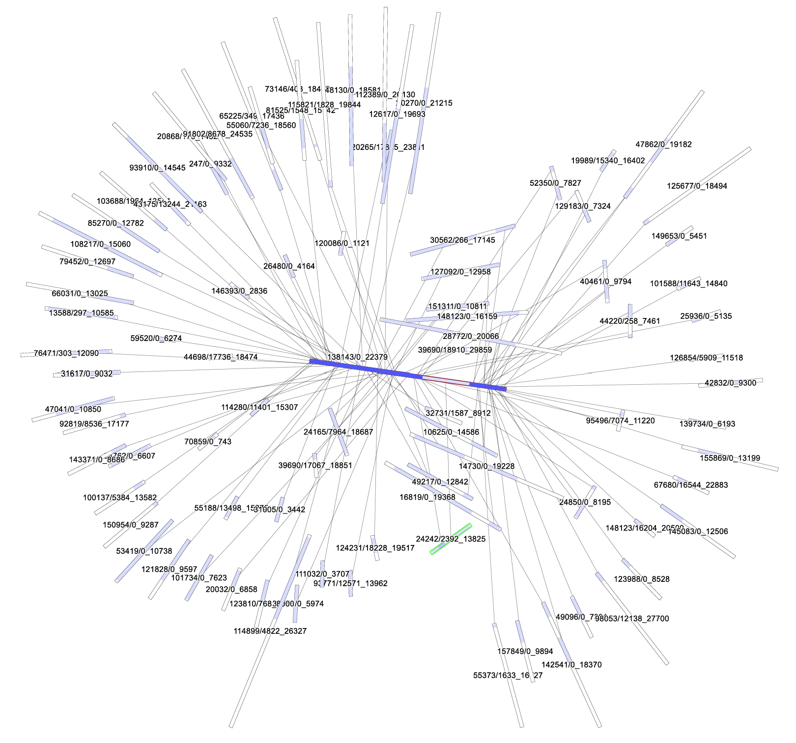 Figure S1: Graph of the pairwise alignments of read 138143/0_22379, approximatively at the center of the graph (with a red outline) to the other reads of the PBcR E. coli dataset. Blue color indicates aligned regions. Due to transparency, a darker blue color indicates multiple alignments in the same region of the read. A region of 1381343/0_22379 is shown in light blue color, while the rest is darker. Interactive inspection of the graph using the GUI of GfaViz revealed that a single read aligns to that region, namely read 24242/2392_13825. To this a green outline was added.
http://www.cbcb.umd.edu/software/PBcR/data/selfSampleData.tar.gz
S1.2 Contig graph reads alignment visualization
GFA 2 allows to record the alignment of reads to contigs using fragment lines. These alignments provide information about the reads which, in the assembly, contributed to the contig. A visual inspection or the representation can be useful, for example, to understand which regions of a contig have a low support by the reads. In a classical visualization of the reads (i.e. pileup), alignments are visualized with respect to a linear reference only (i.e. each contig, separately).
GfaViz allows to visualize the aligned regions in the context of the assembly graph structure. An example is given in Fig. S2. Using the interactive mode it is possible, e.g., to identify the reads aligned to a particular region of the graph. Also in this case, the saturation of the color in a region of the read is higher, whenever multiple reads align to that region. The aligned reads are represented by green and red lines. Their color indicates the relative orientation of the read to the contig (green for reads from the forward strand, red for reads from the reverse strand).
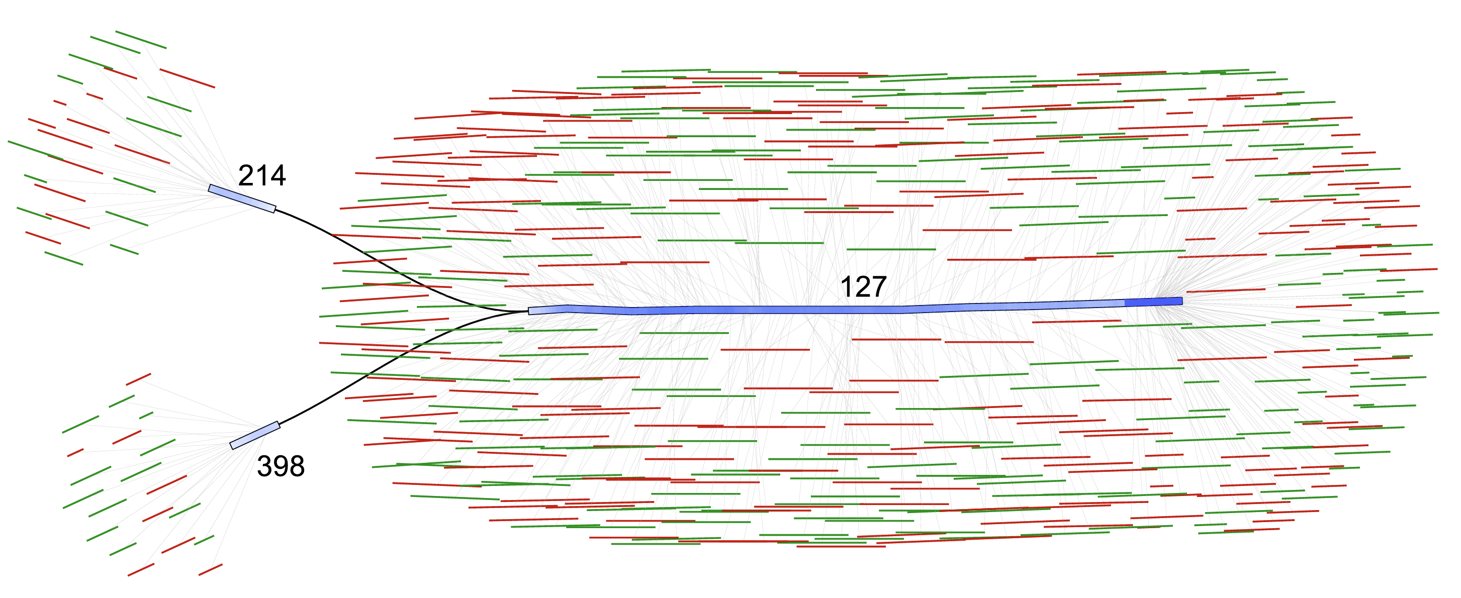 Figure S2: Example of reads-to-contigs alignment graph. A connected components of the Abyss2 contig graph of the GAGE S. aureus dataset, consisting of 3 contigs (214, 398, 127). The reads aligned to the contigs are represented by fragment lines in GFA 2 and visualized as green lines (forward strand) or red lines (reverse strand). The alignment region on the contig is highlighted in blue.
S2 Application examples: Materials and Methods
S2.1 Scaffolding graph and reads-to-contigs alignment graph
2.1.1 Source data
The Staphylococcus aureus dataset of the GAGE Project (Salzberg et al., 2012) was downloaded from the GAGE website1. The readset consists of two Illumina libraries, after correction with ALLPATHS (Maccallum et al., 2009). It includes a fragment library with reads of 101 bp, and a short jump (insert size: 3.5 kbp) mate pair library with reads of length 37 bp.
1http://gage.cbcb.umd.edu/data/Staphylococcus_aureus/Data.allpathsCor.tgz
2.1.2 Assembling of the S. aureus dataset
The S. aureus reads were assembled using Abyss v.2.1.0 (Jackman et al., 2017). The parameters and options for the assembly were the same as used in the GAGE project2 (Salzberg et al., 2012) with the addition of the option graph=ga2.
2http://gage.cbcb.umd.edu/data/Staphylococcus_aureus/Assembly.tgz (file:ABySS2/run.sh)
S2.1.3 Gap information for the scaffolding graph
The assembly graph of the scaffold sequences is output as GFA 2 by the Abyss assembler when using the option graph=ga2. This graph contains dovetail overlaps between pairs of scaffolds, but has no lines describing the gaps. Thus, to obtain a complete scaffolding graph, the abyss- to- dot tool with the options - - ga2 - - estimate was applied to the DOT file containing distance estimates output by abyss- scaffold. The gap lines in the output of abyss- to- dot were added to the assembly graph.
S2.1.4 Visualization of the scaffolding graph
The graph was visualized using GfaViz, using the default layout (Stress Minimization, with default parameters) and the scaffoldling.style stylesheet. The stylesheet specifies that gaps shall be considered as edges in the layout computation (option - - gaps- as- edges). Additionally, it sets the color for gaps of positive size to green and for gaps of negative size to red. Due to space limitations in (Fig. 1a) of the main text, only a part of the largest component of the graph is shown. The entire graph is displayed as Fig. S3.
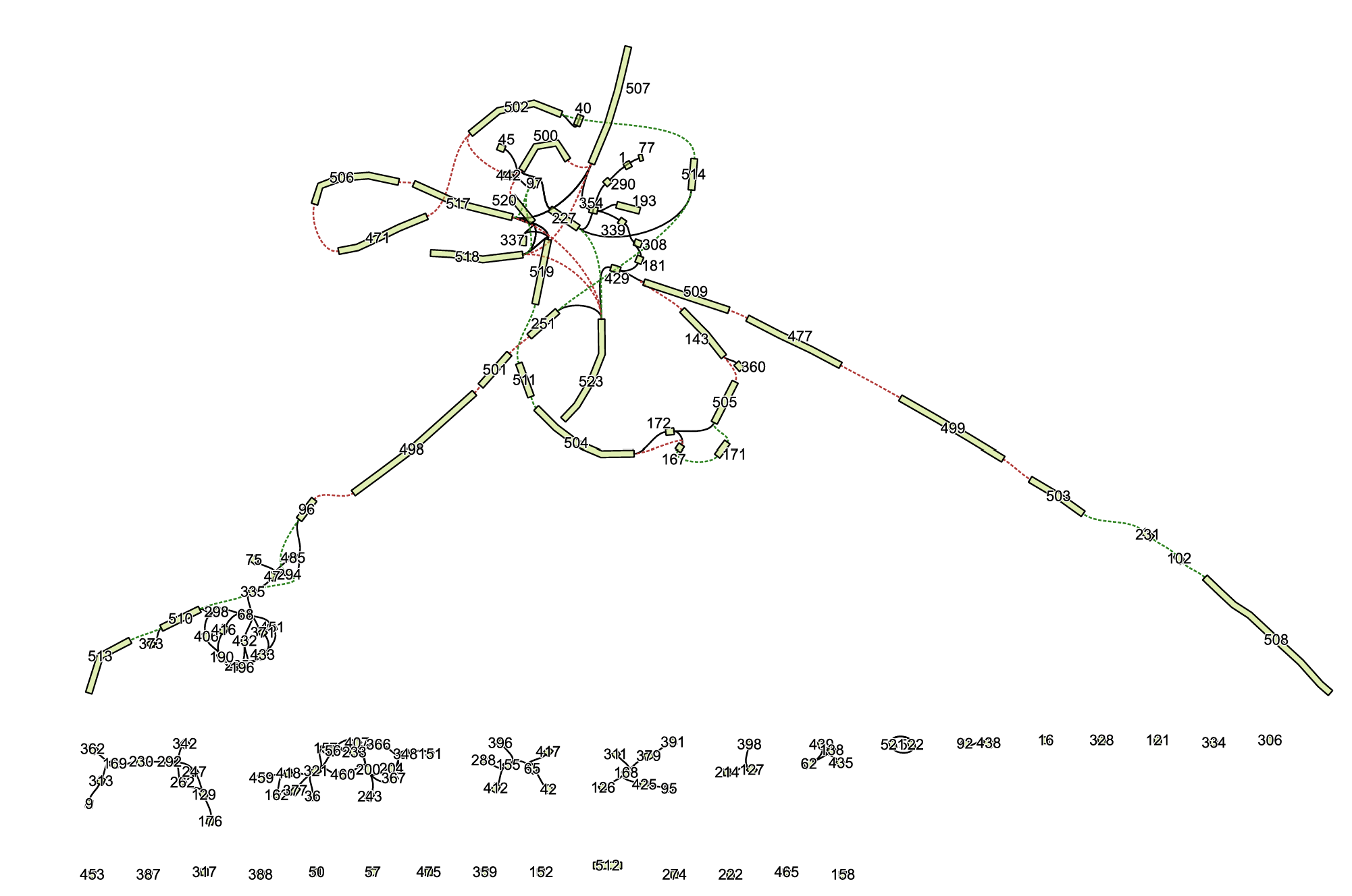 Figure S3: Complete scaffolding graph of the S. aureus assembly, of which a part is shown in Fig. 1a. The contigs are represented by light green polygons. Gaps are represented by dotted lines of different colors: green for gaps of positive size and red for gaps of negative size. Dovetail overlaps of the contigs are represented by black lines.
S2.1.5 Alignments of reads to the contigs
In order to create an example of a visualization of alignments of reads to contigs, a connected component (contigs 214, 398 and 127) was extracted from the GFA 2 contig graph of the S. aureus dataset using GfaPy v.1.0 (Gonnella and Kurtz, 2017). The fragment library was mapped against the contig using bwa mem v.0.7.15 (Li, 2013) with default parameters. Unaligned reads were removed from the SAM output using samtools v.1.4.1 (Li et al., 2009). Fragment lines describing the alignments of the reads to the contigs in the connected component were obtained from the resulting SAM file using a custom Python script (sam_to_ga2. py) and added to the GFA 2 file.
S2.1.6 Visualization of the reads-to-contigs alignment graph
The reads- to- contigs graph was visualized with GfaViz, using the FMMM layout and the reads2contigs.style stylesheet. The stylesheet increases the distance of fragments to segments (because of the large number of fragments) and enables fragment highlights, which show the regions of the segments aligned to the external sequences.
S2.2 Variation graph
S2.2.1 Source data
S2.2.1 Source dataA sample variation graph of vg (Garrison et al., 2018), representing variants of the H. sapiens major histocompatibility complex HLA- B, was obtained from the vg Github repository3. The vg view tool of vg v.1.11.0 was used to create a graph in GFA 1 format.
3https://github.com/vgteam/vg/blob/master/test/graphs/not-simple.vg
S2.2.2 Visualization of the variation graph
S2.2.2 Visualization of the variation graphThe variation graph was visualized using GfaViz, using the default layout (stress minimization) with default parameters and using the stylesheet variation.style. The stylesheet defines the colors of the groups and switches on the visualization of the sequences as labels of segments (option - - seg- label- seq).
S2.3 Metagenomic binning graph
S2.3.1 Simulated metagenomic dataset
S2.3.1 Simulated metagenomic datasetA simulated metagenomic dataset, consisting of 20 million simulated Illumina read pairs (read length 80 bp) from 10 source genomes, was prepared as described in Wu et al. (2014). Thereby the source genomes are the 10 bacterial genomes with a length between 2.2 Mbp and 7.8 Mbp indicated in the Supplementary Materials (Table S1) of Wu et al. (2014). The relative abundances used for the simulation were set to the values (between 3.0% and 37.9%) indicated in the same table. The reads were simulated using MetaSim (Richter et al., 2008). The empirical error model for the reads was obtained from the MetaSim website4.
4https://ab.inf.uni-tuebingen.de/software/metasim/errormodel-80bp.mconf/at_download/file
S2.3.2 Assembling of the metagenomic dataset
S2.3.2 Assembling of the metagenomic datasetThe simulated metagenomic dataset was assembled using SPAdes v.3.13.0 (Bankevich et al., 2012) and the options - - meta for metagenome assembly and - - only- assembler to skip the reads error correction stage, which requires quality scores, not provided by MetaSim.
S2.3.3 Binning of the metagenomic assembly
The scaffolds output by SPAdes (scaffolds.fasta) were classified into bins by MaxBin v.2.2.5 (Wu et al., 2014), using default parameters. The description lines of the output Fasta files for each bin were used to obtain a list of the scaffolds in each bin. Using a custom Python script maxbin_to_gfa.py, based on Gfapy v.1.0 (Gonnella and Kurtz, 2017), the GFA 1 scaffolds graph output of SPAdes was converted to GFA 2 and the binning information was coded as GFA 2 unordered groups.
S2.3.4 Visualization of the metagenomic binning graph
The metagenomic binning graph was visualized using GfaViz, using the FMMM layout (option - - fmmm) and the metagenome.style stylesheet. This sets the colors for the group outlines, switches on the group labels and increases their font size to 36.
S2.4 Alignment graph of long reads
S2.4.1 Source data
The E. coli K12 sample dataset of the PacBio correction pipeline PBCR (Berlin et al., 2015) was obtained from the PBCR website. It consists of a random subset of data obtained using the PacBio RS II sequencer with P5- C3 chemistry and a single SMRTcell.
S2.4.2 Pairwise reads alignments
Alignments among the Pacbio reads were computed using minimap2 v.2.0 (Li, 2018), using the options - x ava- pb. A custom Python script paf2gfa2. py, collects the alignments for a given read (138143/0_22379) and converts them to GFA 2.
S2.4.3 Visualization of the long reads alignment graph
The alignment graph of read 138143/0_22379 to other reads in the PBCR E. coli dataset was visualized using GfaViz with the default layout (stress minimization) and the longreads.style stylesheet. The stylesheet specifies that segments are visualized by straight lines (option - seg- max- sub 1) and turns on the visualization of the aligned regions of the segments (option - - edges- highlights- show).
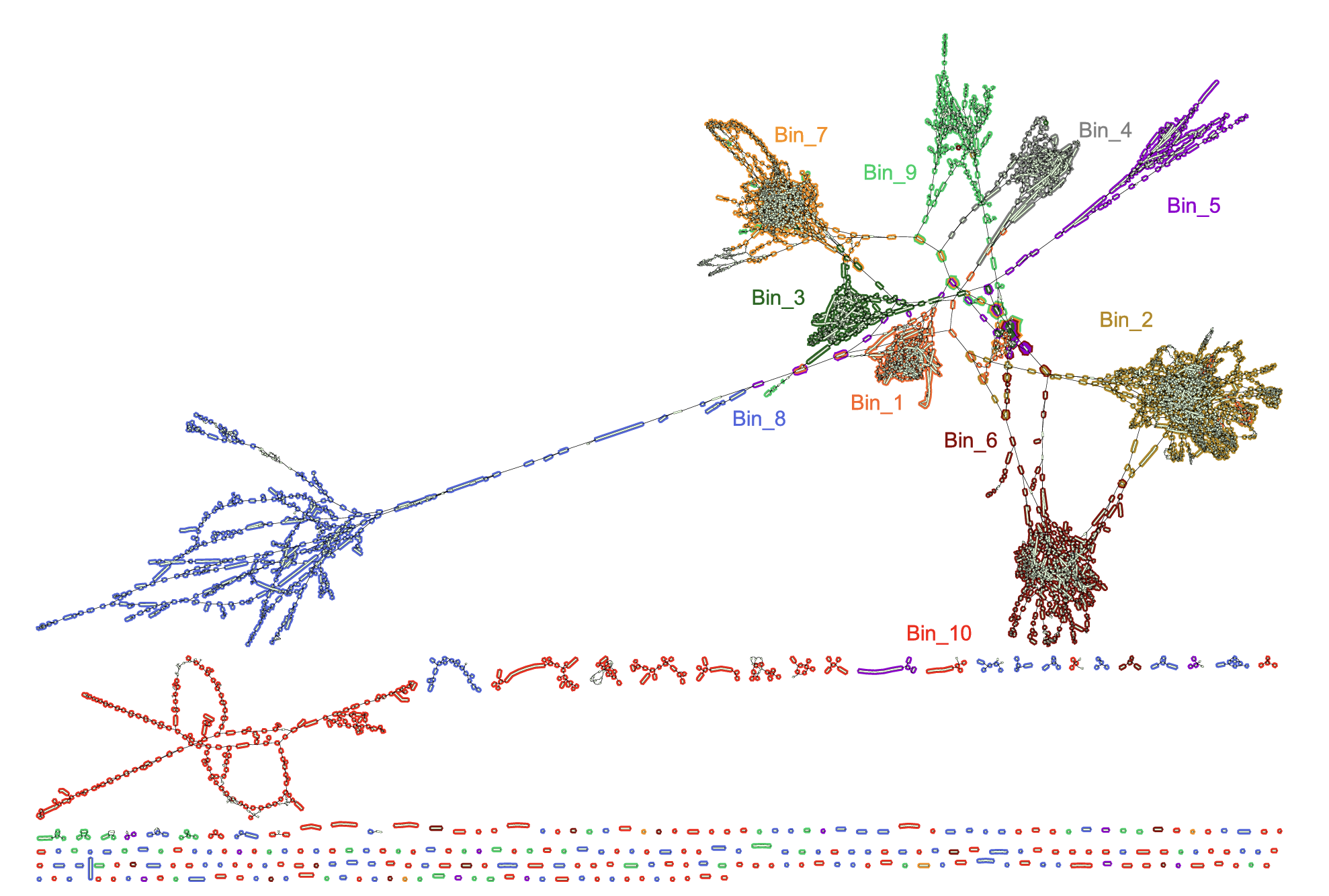 Figure S4: Complete metagenomic binning graph of the simulated metagenomic dataset, of which a part is shown in Fig. 1b. The bins are represented by colored outlines.
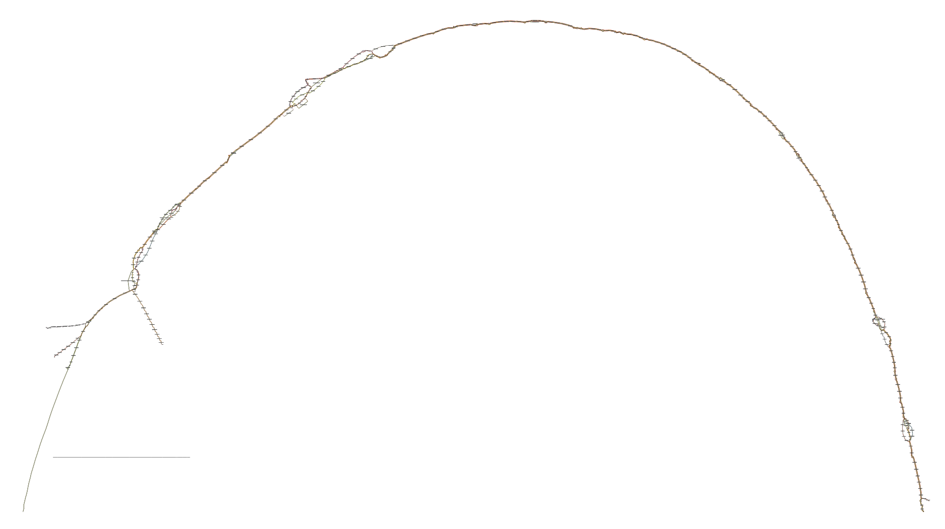 Figure S5: Complete variation graph of the HLA-B locus, of which a part is shown in Fig. 1c.
S3 Application examples: Complete graphs
Due to space limitation, the main text only shows visualizations of parts of the graphs. The corresponding complete graphs are shown in this section.
The complete scaffolding graph, of which a part is shown in Fig. 1a, is displayed in Fig. S3. The complete metagenomic binning graph, of which a part is shown in Fig. 1b is displayed in Fig. S4. The complete variation graph, of which a part is shown in Fig. 1c is displayed in Fig. S5.
References
Bankevich, A., Nurk, S., Antipov, D., Gurevich, A. a., Dvorkin, M., Kulikov, A. S., Lesin, V. M., Nikolenko, S. I., Pham, S., Prjibelski, A. D., Pyshkin, A. V., Sirotkin, A. V., Vyahhi, N., Tesler, G., Alekseyev, M. a., and Pevzner, P. a. (2012). SPAdes: a new genome assembly algorithm and its applications to single- cell sequencing. J. Comput. Biol., 19(5), 455- 77. Berlin, K., Koren, S., Chin, C.- S., Drake, J. P., Landolin, J. M., and Phillippy, A. M. (2015). Assembling large genomes with single- molecule sequencing and locality- sensitive hashing. Nat. Biotechnol., 33(6), 623- 630. Garrison, E., Siren, J., Novak, A. M., Hickey, G., Eizenga, J. M., Dawson, E. T., Jones, W., Garg, S., Markello, C., Lin, M. F., Paten, B., and Durbin, R. (2018). Variation graph toolkit improves read mapping by representing genetic variation in the reference. Nat. Biotechnol., 36(9), 875- 881. Gonnella, G. and Kurtz, S. (2017). Gfayp: a flexible and extensible software library for handling sequence graphs in Python. Bioinformatics, 33(19), 3094- 3095. Jackman, S. D., Vandervalk, B. P., Mohamadi, H., Chu, J., Yeo, S., Hammond, S. A., Jahesh, G., Khan, H., Coombe, L., Warren, R. L., and Birol, I. (2017). ABySS 2.0: resource- efficient assembly of large genomes using a Bloom filter. Genome Res., 27(5), 768- 777. Li, H. (2013). Aligning sequence reads, clone sequences and assembly contigs with BWA- MEM. arXiv:1303.3997v1 [q- bio.GN]. Li, H. (2018). Minimap2: pairwise alignment for nucleotide sequences. Bioinformatics, 34(18), 3094- 3100. Li, H., Handsaker, B., Wysoker, A., Fennell, T., Ruan, J., Homer, N., Marth, G., Abecasis, G., and Durbin, R. (2009). The Sequence Alignment/Map format and SAMtools. Bioinformatics, 25(16), 2078- 9. Maccallum, I., Przybylski, D., Gnerre, S., Burton, J., Shlyakhter, I., Gnirke, A., Malek, J., McKernan, K., Ranade, S., Shea, T. P., Williams, L., Young, S., Nusbaum, C., and Jaffe, D. B. (2009). ALLPATHS 2: small genomes assembled accurately and with high continuity from short paired reads. Genome Biol., 10(10), R103. Richter, D. C., Ott, F., Auch, A. F., Schmid, R., and Huson, D. H. (2008). Metasima sequencing simulator for genomics and metagenomics. PLOS ONE, 3(10), 1- 12. Salzberg, S. L., Phillippy, A. M., Zimin, A., Puiu, D., Magoc, T., Koren, S., Treangen, T. J., Schatz, M. C., Delcher, A. L., Roberts, M., Marcais, G., Pop, M., and Yorke, J. a. (2012). GAGE: A critical evaluation of genome assemblies and assembly algorithms. Genome Res., 22(3), 557- 67. Wu, Y.- W., Tang, Y.- H., Tringe, S. G., Simmons, B. A., and Singer, S. W. (2014). Maxbin: an automated binning method to recover individual genomes from metagenomes using an expectation- maximization algorithm. Microbiome, 2(1), 26.